library(tidyverse)
library(rstan)
library(bayesplot)
library(knitr)
library(loo)
library(ggExtra)

# load other packages as neededHW 04: Hierarchical models
Modeling disease progression in glaucoma
Due date
This assignment is due on Thursday, March 25 at 11:45am. To be considered on time, the following must be done by the due date:
- Final
.qmdand.pdffiles pushed to your GitHub repo - Final
.pdffile submitted on Gradescope
Getting started
Go to the biostat725-sp25 organization on GitHub. Click on the repo with the prefix hw-04. It contains the starter documents you need to complete the homework.
Clone the repo and start a new project in RStudio. See the AE 01 instructions for details on cloning a repo and starting a new project in R.
Packages
The following packages are used in this assignment:
Introduction
This homework will use data from the Rotterdam Ophthalmic Data Repository. Glaucoma is the leading cause of irreversible blindness world wide with over 60 million glaucoma patients as of 2012. Since impairment caused by glaucoma is irreversible, early detection of disease progression is crucial for effective treatment. Patients with glaucoma are routinely followed up and administered visual fields, a functional assessment of their vision. After each visual field test their current disease status is reported as a mean deviation value, measured in decibels (dB). A lower mean deviation indicates worse vision. Data was collected for each eye longitudinally and disease progression is estimated as the slope across time (dB/year). The data is available in dat-hw4.rds and we will use the following variables.
eye: integer, indicating the unique eye-level study id number.mean_deviation: continuous, MD value for each eye \(i\) and time \(t\).time: continuous, time from baseline visual field (years).age: integer, age of the patient at baseline (years).iop: continuous, intraocular pressure measured at baseline (mm Hg).baseline_md: continuous, baseline MD value for eye \(i\).
The dataset can be loaded as follows.
dat_hw4 <- readRDS("dat-hw4.rds")Exercises 1-6
Define \(Y_{it}\) as the MD value for eye \(i\) (\(i = 1,\ldots,n\)) and visit \(t\) (\(t = 1,\ldots, n_i\)), and \(X_{it}\) is the follow-up time, such that \(X_{i0} = 0\). Researchers are interested in estimating the eye-specific slopes for our sample to identify which patients are progressing (i.e., slope less than 0). To estimate these eye-specific slopes, researchers would like to fit the following model:
\[\begin{align*} Y_{it} | \boldsymbol{\Omega}, \boldsymbol{\theta}_i &\stackrel{iid}{\sim} N\left(\beta_{0i} + \beta_{1i}X_{it}, \sigma^2\right),\\ \beta_{0i} &= \beta_{0} + \theta_{0i}\\ \beta_{1i} &= \beta_{1} + \theta_{1i}\\ \boldsymbol{\theta}_i | \boldsymbol{\Sigma} &\stackrel{iid}{\sim} N_2(\mathbf{0}_2,\boldsymbol{\Sigma}),\quad \boldsymbol{\Sigma} = \begin{bmatrix} \tau_{0}^2 & \rho \tau_0 \tau_1\\ \rho \tau_0 \tau_1 & \tau_1^2\\ \end{bmatrix}\\ \boldsymbol{\Omega} &\sim f(\boldsymbol{\Omega}), \end{align*}\] where \(\boldsymbol{\theta}_i = (\theta_{0i},\theta_{1i})\) and \(\boldsymbol{\Omega} = (\beta_0, \beta_1, \sigma^2, \boldsymbol{\Sigma})\). For priors, the researchers want to decompose the covariance structure, such that \(\boldsymbol{\Sigma} = \mathbf{D}\mathbf{L}\mathbf{L}^\top\mathbf{D}\), where \(\mathbf{D}\) is a diagonal matrix with the standard deviations \((\tau_0,\tau_1)\) on the diagonals. and \(\mathbf{L}\) is the lower triangular Cholesky of the correlation matrix, \(\boldsymbol{\Phi} = \mathbf{L}\mathbf{L}^\top\).
Exercise 1
Fit the eye-specific intercept and slope model to the glaucoma data using the conditional model given above. For priors use \({\beta}_j \sim N(0,3^2)\) for \(j = 0,1\), \(\sigma \sim \text{Half-Normal}(0,3^2)\), \(\tau_{j} \sim \text{Half-Normal}(0, 3^2)\) for \(j =0,1\), and \(\mathbf{L} \sim LKJ(\eta)\), with \(\eta = 1\). Assess model convergence and perform a posterior predictive check.
Notes: This model may take a bit longer to run, one way to speed this up is to run options(mc.cores = 4) to run the chains in parallel. You may also want to only save parameters that you will need in subsequent exercises, by specifying sampling(..., pars = c("parameters you don't want to save"), include = FALSE). This will make the model fit object must smaller. Finally, it is possible that the model will need to be run a bit longer for convergence, so you may need to increase iter.
Exercise 2
Explore the posterior mean estimates for the eye-specific slopes, \(\beta_{1i}\). Plot the posterior mean estimates of \(\beta_{1i}\) against the eye-specific slopes obtained from ordinary least squares (OLS) regression. How do the slopes compare from the two models? Hint: It may be helpful to plot a line with zero intercept and slope one.
Exercise 3
Summarize the posterior distributions of the population parameters \(\beta_0\) and \(\beta_1\). Interpret the posterior means for each parameter in the context of the scientific problem.
Exercise 4
Explore the correlation between eye-specific intercepts (\(\beta_{0i}\)) and slopes (\(\beta_{1i}\)). Create a scatter plot to examine their relationship. Does their appear to be a relationship? To help answer this question also create examine the posterior distribution for \(\rho\) and comment on how it relates to the scatter plot.
Exercise 5
Compute the posterior probability of progression for each participant, \(p_i = P(\beta_{1i} < 0 | \mathbf{Y})\). Define progression as \(prog_i = 1(p_i > 0.95)\) Plot the \(prog_i\) versus eye-specific baseline variables, including age, IOP, and baseline MD. Are any baseline characteristics associated with progression?
Exercise 6
Suppose we have a new eye, \(\mathbf{Y}_{i^*} = \left(Y_{i^*1},\ldots,Y_{i^*n_{i^*}}\right)\), that was not used to train the original data. We are interested in predicting their next visual field at time \(X_{i^*t^*}\), where \(t^* = (n_{i^*} + 1)\). The posterior predictive distribution is given by:
\[\begin{align*} f\left(Y_{i^*t^*} | \mathbf{Y}_{i^*}, \mathbf{Y}\right) &= \int f\left(Y_{i^*t^*},\boldsymbol{\Omega},\boldsymbol{\theta}_{i^*} | \mathbf{Y}_{i^*}, \mathbf{Y}\right) d\boldsymbol{\Omega}d\boldsymbol{\theta}_{i^*}\\ &= \int f\left(Y_{i^*t^*} | \boldsymbol{\Omega},\boldsymbol{\theta}_{i^*} , \mathbf{Y}_{i^*}, \mathbf{Y}\right) f\left(\boldsymbol{\Omega},\boldsymbol{\theta}_{i^*} | \mathbf{Y}_{i^*}, \mathbf{Y}\right) d\boldsymbol{\Omega}d\boldsymbol{\theta}_{i^*}\\ &= \int \underbrace{f\left(Y_{i^*t^*} | \boldsymbol{\Omega},\boldsymbol{\theta}_{i^*}\right)}_{\text{Likelihood}} \underbrace{f\left(\boldsymbol{\theta}_{i^*} |\boldsymbol{\Omega}, \mathbf{Y}_{i^*}\right)}_{\text{Eye-Specific Posterior}}\underbrace{f\left(\boldsymbol{\Omega}|\mathbf{Y}\right)}_{\text{Posterior}} d\boldsymbol{\Omega}d\boldsymbol{\theta}_{i^*}\\ \end{align*}\]
Similar to the posterior predictive distributions we have worked with before, we can sample from all three of these distributions to obtain samples from the posterior predictive distribution for the the future observation \(Y_{i^*t^*}\). The first distribution is the conditional likelihood, the second distribution is the posterior distribution for a subject-specific parameter (which we derived for the marginal likelihood in the lecture slides), and the third distribution is the posterior.
The new eye has five observation (\(n_{i^*} = 5\)) with the following MD values: \(\mathbf{Y}_{i^*} = (-1.44, -2.01, -1.98, -2.67, -3.01)\) that were observed at the following time points: \((0.00, 0.56, 1.20, 1.80, 2.40)\). Provide the posterior predictive distribution for \(Y_{i^*t^*}\) at three years from baseline (i.e., \(X_{i^*t^*} = 3\)).
Exercises 7-9
When studying the eye-specific slopes from the OLS regressions (given in the figure below), the researchers are concerned that there are some outliers that may actually be clinically realistic. For example, a slope of -3 may be possible in certain types of glaucoma.
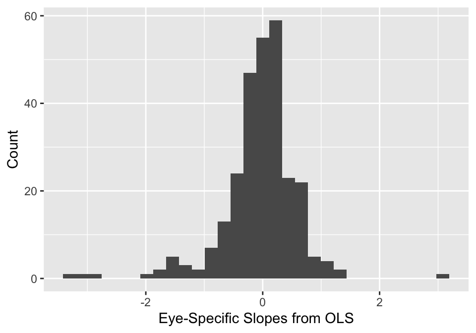
Based on this observation, the researchers would like a more robust model for the eye-specific parameters. They decide to specify a multivariate Student-t distribution: \(\boldsymbol{\theta}_i \stackrel{iid}{\sim} t_{\nu}(\mathbf{0}, \boldsymbol{\Sigma})\). To generate these parameters efficiently, the researchers use the following transformation of standard normal random variables and inverse-\(\chi^2\) random variables, \[\boldsymbol{\theta}_i = \sqrt{\nu v_i}\mathbf{D}\mathbf{L} \mathbf{z}_i,\] where \(\mathbf{z}_i = (z_{i0}, z_{i1})\) and \(z_{ij} \stackrel{iid}{\sim} N(0,1)\), and \(v_i \stackrel{iid}{\sim} \text{Inv-}\chi^2_{\nu}\). Place the following prior on \(\nu \sim \text{Gamma}(2,0.1)\).
Exercise 7
Fit the same model as in Exercise 1, but replace the multivariate Gaussian prior with a multivariate Student-t prior. Assess model convergence and perform a posterior predictive check. Create a scatter plot of the posterior mean eye-specific slopes from the Gaussian and Student-t models. Describe the relationship?
Exercise 8
Examine the posterior distribution of \(\nu\). What does the posterior distribution of \(\nu\) tell us about the appropriateness of the Student-t model, as compared to the Gaussian model?
Exercise 9
Compare the Gaussian and Student-t models using LOO-IC. Which model is preferred? Is this consistent with your answer from Exercise 8?
Submission
You will submit the PDF documents for homeworks, and exams in to Gradescope as part of your final submission.
Warning
Before you wrap up the assignment, make sure all documents are updated on your GitHub repo. We will be checking these to make sure you have been practicing how to commit and push changes.
Remember – you must turn in a PDF file to the Gradescope page before the submission deadline for full credit.
To submit your assignment:
Access Gradescope through the menu on the BIOSTAT 725 Canvas site.
Click on the assignment, and you’ll be prompted to submit it.
Mark the pages associated with each exercise. All of the pages of your homework should be associated with at least one question (i.e., should be “checked”).
Grading
| Component | Points |
|---|---|
| Ex 1 | 10 |
| Ex 2 | 5 |
| Ex 3 | 5 |
| Ex 4 | 5 |
| Ex 5 | 5 |
| Ex 6 | 5 |
| Ex 7 | 8 |
| Ex 8 | 4 |
| Ex 9 | 3 |