AE 01: Posterior estimation using Gibbs sampling

Glaucoma disease progression

Published

January 16, 2025

Due date

Application exercises (AEs) are submitted by pushing your work to the relevant GitHub repo. AEs from Tuesday lectures should be submitted by Friday by 11:59pm ET, and AEs from Thursday lectures should be submitted by Sunday at 11:59pm ET. Because AEs are intended for in-class activities, there are no extensions given on AEs.

This AE is due on Sunday, January 19 at 11:59pm. To be considered on time, the following must be done by the due date:

Final .qmd and .pdf files pushed to your GitHub repo
Note: For homeworks and exams, you will also be required to submit your final .pdf file submitted on Gradescope

Introduction

This AE will go through much of the workflow we will use in the course. The main goal is to demo the use of R and RStudio, which we will be using throughout the course both to learn the statistical concepts discussed in the course and to analyze real data and come to informed conclusions.

Learning goals

By the end of the AE, you will…

Be familiar with the workflow using RStudio and GitHub
Gain practice writing a reproducible report using Quarto
Practice version control using GitHub
Perform Gibbs sampling for Bayesian linear regression and compute some basic summaries

Getting Started

Clone the repo & start new RStudio project

Go to the course organization at github.com/biostat725-sp25 organization on GitHub.
Click on the repo with the prefix ae-01-. It contains the starter documents you need to complete the AE.
Click on the green CODE button, select Use SSH (this might already be selected by default, and if it is, you’ll see the text Clone with SSH). Click on the clipboard icon to copy the repo URL.
- See the HW 00 instructions if you have not set up the SSH key or configured git.
In RStudio, go to File $\to$ New Project $\to$ Version Control $\to$ Git.
Copy and paste the URL of your assignment repo into the dialog box Repository URL. Again, please make sure to have SSH highlighted under Clone when you copy the address.
Click Create Project, and the files from your GitHub repo will be displayed in the Files pane in RStudio.
Click ae-01-mcmc.qmd to open the template Quarto file. This is where you will write up your code and narrative for the AE.

R and R Studio

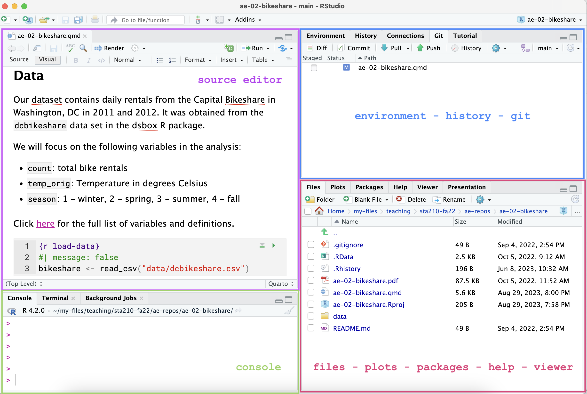
Below are the components of the RStudio IDE.

Below are the components of a Quarto (.qmd) file.

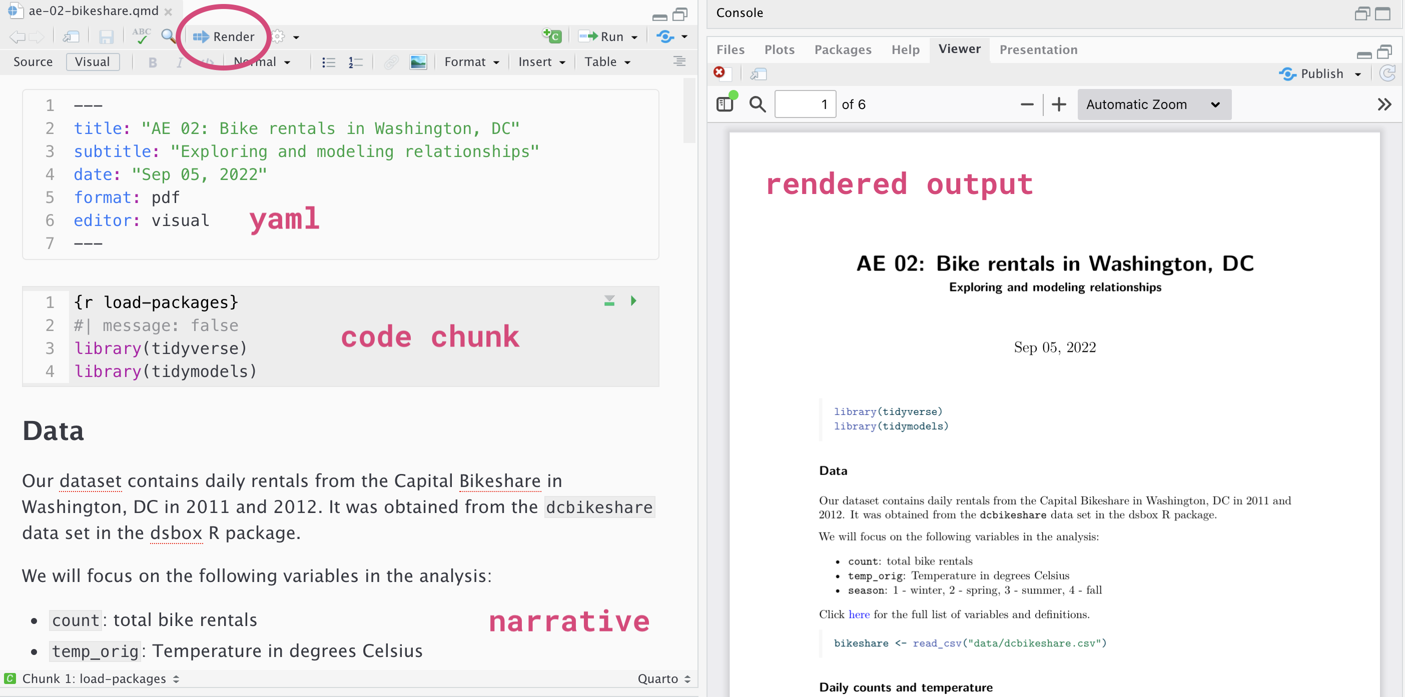
Screenshot of Quarto document and rendered PDF.

YAML

The top portion of your Quarto file (between the three dashed lines) is called YAML. It stands for “YAML Ain’t Markup Language”. It is a human friendly data serialization standard for all programming languages. All you need to know is that this area is called the YAML (we will refer to it as such) and that it contains meta information about your document.

Important

Open the Quarto (.qmd) file in your project, change the author name to your name, and render the document. Examine the rendered document.

Committing changes

Now, go to the Git pane in your RStudio instance. This will be in the top right hand corner in a separate tab.

If you have made changes to your Quarto (.qmd) file, you should see it listed here. Click on it to select it in this list and then click on Diff. This shows you the difference between the last committed state of the document and its current state including changes. You should see deletions in red and additions in green.

If you’re happy with these changes, we’ll prepare the changes to be pushed to your remote repository. First, stage your changes by checking the appropriate box on the files you want to prepare. Next, write a meaningful commit message (for instance, “updated author name”) in the Commit message box. Finally, click Commit. Note that every commit needs to have a commit message associated with it.

You don’t have to commit after every change, as this would get quite tedious. You should commit states that are meaningful to you for inspection, comparison, or restoration.

In the first few assignments we may tell you exactly when to commit and in some cases, what commit message to use. As the semester progresses we will let you make these decisions.

Push changes

Now that you have made an update and committed this change, it’s time to push these changes to your repo on GitHub.

In order to push your changes to GitHub, you must have staged your commit to be pushed. click on Push.

Now let’s make sure all the changes went to GitHub. Go to your GitHub repo and refresh the page. You should see your commit message next to the updated files. If you see this, all your changes are on GitHub and you’re good to go!

R packages

We will begin by loading R packages that we will use in this AE.

library(tidyverse)    # data wrangling and visualization
library(tidymodels)   # broom and yardstick package
library(knitr)        # format output
library(skimr)        # quickly calculate summary statistics
library(mvtnorm)      # multivariate normal rng

Data

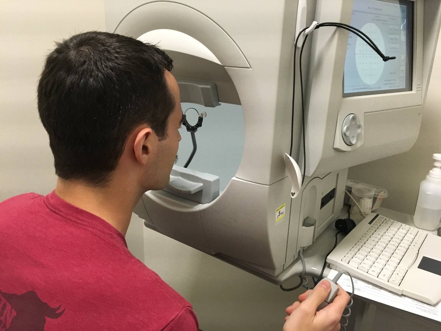
The data are on patients with glaucoma from the Rotterdam Ophthalmic Data Repository. Glaucoma is the leading cause of irreversible blindness world wide with over 60 million glaucoma patients as of 2012. Since impairment caused by glaucoma is irreversible, early detection of disease progression is crucial for effective treatment. Patients with glaucoma are routinely followed up and administered visual fields, a functional assessment of their vision. After each visual field test their current disease status is reported as a mean deviation value, measured in decibels (dB). A lower mean deviation indicates worse vision. An important predictor of disease progression is intraocular pressure (IOP), the pressure of fluids inside your eye.

We will focus on two variables:

iop: intraocular pressure, measured in millimeters of mercury (mmHg)
progression: rate of disease progression, measured as the number dB lost per year (dB/year)

The goal of this analysis is to use the IOP to understand variability in disease progression in glaucoma patients. The data is available in the ae-01- repo and is called glaucoma.rds.

glaucoma <- readRDS(file = "glaucoma.rds")
glimpse(glaucoma)

Rows: 139
Columns: 7
$ id          <int> 1, 2, 3, 4, 5, 6, 7, 8, 9, 10, 11, 12, 13, 14, 15, 16, 17,…
$ age         <dbl> 51.55616, 76.78356, 46.38356, 42.56712, 68.36438, 56.61644…
$ sex         <chr> "F", "F", "F", "M", "F", "F", "F", "F", "M", "M", "M", "M"…
$ iop         <dbl> 10.333333, 11.750000, 14.666667, 5.333333, 12.666667, 18.3…
$ baseline_md <dbl> -7.69, -5.38, -22.05, -13.99, -13.02, -7.13, -2.69, -9.43,…
$ severity    <chr> "Moderate", "Mild", "Severe", "Severe", "Severe", "Moderat…
$ progression <dbl> -0.190141797, -0.055098961, 0.431682497, 0.218545250, 0.08…

Exploratory data analysis

Let’s begin by examining the univariate distributions of the disease progression and IOP. The code to visualize and calculate summary statistics for progression is below.

ggplot(data = glaucoma, aes(x = progression)) + 
  geom_histogram() +
  labs(x = "Disease progression (db/year)", 
       y = "Count",
       title = "Disease progression in glaucoma patients")

`stat_bin()` using `bins = 30`. Pick better value with `binwidth`.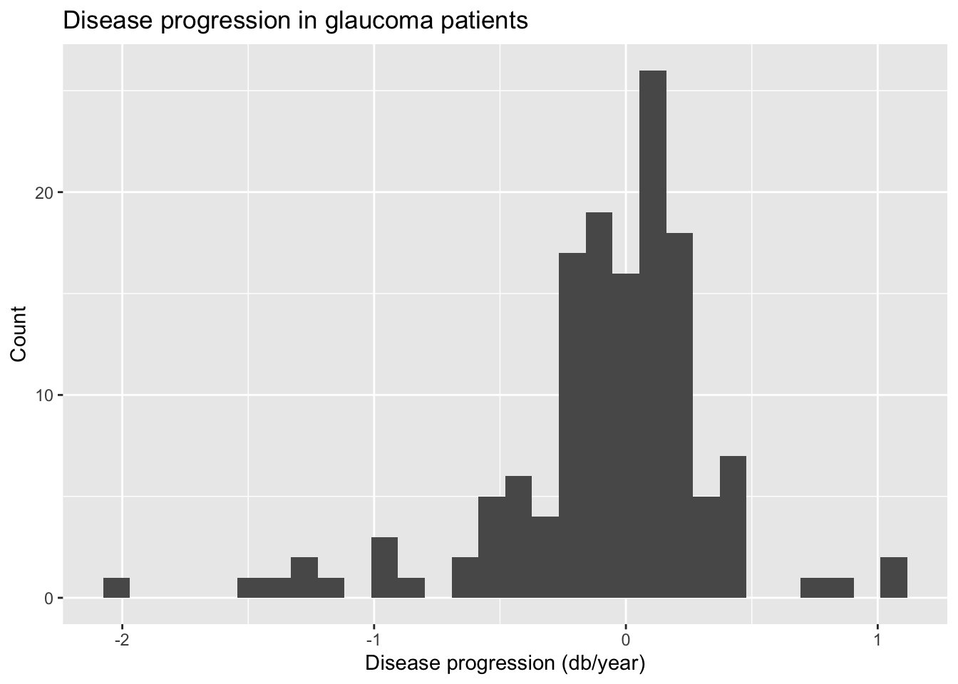

glaucoma |>
  summarise(min = min(progression), q1 = quantile(progression, 0.25), 
            median = median(progression), q3 = quantile(progression, 0.75), 
            max = max(progression), mean = mean(progression), sd = sd(progression)) |>
  kable(digits = 3)

min	q1	median	q3	max	mean	sd
-1.981	-0.207	-0.022	0.149	1.107	-0.079	0.441

Posterior estimation

You want to fit a model of the form

$p r o g r e s s i o n_{i} = β_{0} + β_{1} i o p_{i} + ϵ, ϵ \sim N (0, σ^{2}) .$

We can obtain samples from the posterior distribution for the regression parameters using the specification from the slides. We define the data objects needed for posterior estimation.

X <- cbind(1, glaucoma$iop) # covariate matrix
Y <- glaucoma$progression # outcome definition
p <- ncol(X) - 1 # number of covariates (excluding the intercept)
n <- length(Y) # number of observations

We will then define hyperparameters for the priors. We will choose a weakly informative prior. We will discuss more about priors in subsequent lectures. For now, we will place the following priors: $β \sim N (β_{0}, σ_{β}^{2} I_{2})$ and $σ^{2} \sim Inv-Gamma (a, b)$ .

sigma_beta2 <- 10
beta0 <- rep(0, p + 1)
a <- 3 
b <- 1

We can now obtain samples from the posterior using Gibbs sampling. Let’s set $S = 5, 000$ . We begin by randomly initializing $σ^{2}$ .

S <- 5000
sigma2 <- exp(rnorm(1)) # initial value

Run a for loop over samples.

samples <- NULL
for (s in 1:S) {
  
  ###Sample from full conditional for beta
  var_beta <- chol2inv(chol(t(X) %*% X / sigma2 + diag(p + 1) / sigma_beta2))
  mean_beta <- var_beta %*% (beta0 / sigma_beta2 + t(X) %*% Y / sigma2)
  beta <- as.numeric(rmvnorm(1, mean_beta, var_beta))
  
  ###Sample from full conditional for sigma2
  quadratic <- as.numeric(t(Y - X %*% beta) %*% (Y - X %*% beta))
  sigma2 <- 1 / rgamma(1, shape = a + n / 2, rate = b + quadratic / 2)
  
  ###Save samples
  samples <- rbind(samples, c(beta, sigma2))
  
}

Insepction of Gibbs sampler

We can begin by inspecting the posterior density and traceplots.

dat.fig <- data.frame(
  parameter = rep(c("beta[0]", "beta[1]", "sigma^2"), each = S),
  index = rep(1:S, 3),
  value = as.numeric(samples)
)
ggplot(dat.fig, aes(x = value)) +
  geom_density(lwd = 1.5) +
  facet_grid(. ~ parameter, labeller = label_parsed, scales = "free_x") +
  ylab("Density") +
  xlab("Parameter value")
ggplot(dat.fig, aes(x = index, y = value)) + 
  geom_line(lwd = 0.5) + 
  facet_grid(. ~ parameter, labeller = label_parsed, scales = "free_x") + 
  ylab("Parameter value") +
  xlab("Sample index")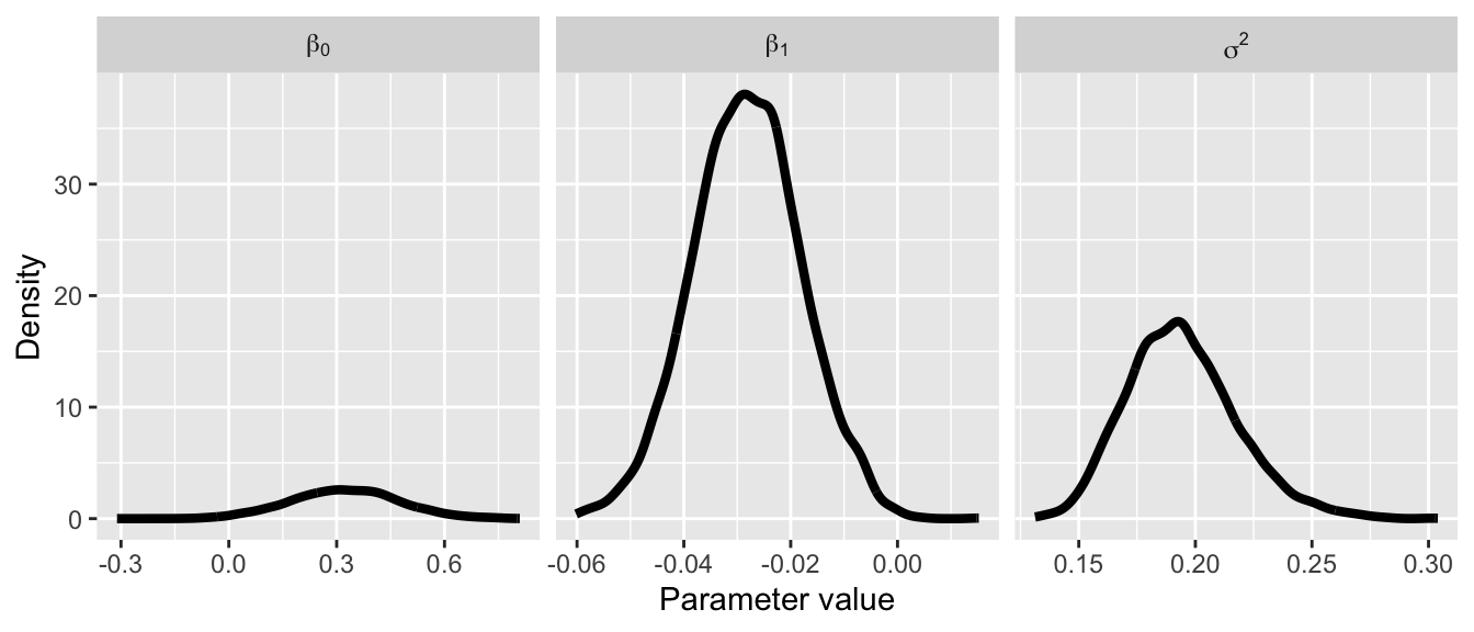

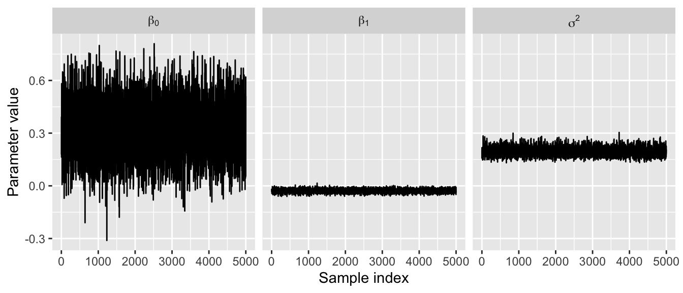
The traceplots do not exhibit much autocorrelation, indicating our samples have properly converged. We will dive into this much more in subsequent lectures.

Exercises

Exercise 1

Compute the posterior mean and standard deviation for the intercept, slope, and measurement error. Provide an interpretation for each of these parameter estimates.

Answer:

# add code here

Exercise 2

Compute a 95% confidence interval for the regression slope. Provide an interpretation for this confidence interval.

Answer:

# add code here

Exercise 3

Compute a one-sided Bayesian p-value for the regression slope: $P (β_{1} < 0)$ . Interpret the results in plain English. Is intraocular pressure associated with disease progression?

Answer:

# add code here

Important

To submit the AE:

Render the document to produce the PDF with all of your work from today’s class.
Push all your work to your AE repo on GitHub. You’re done! 🎉