library(tidyverse)
library(rstan)
library(bayesplot)
library(knitr)
library(loo)
library(MLMusingR)
library(kableExtra)
library(LaplacesDemon)

# load other packages as neededHW 03: Going beyond linear regression
Hospital length of stay post lung cancer surgery
Due date
This assignment is due on Thursday, February 27 at 11:45am. To be considered on time, the following must be done by the due date:
- Final
.qmdand.pdffiles pushed to your GitHub repo - Final
.pdffile submitted on Gradescope
Getting started
Go to the biostat725-sp25 organization on GitHub. Click on the repo with the prefix hw-03. It contains the starter documents you need to complete the homework.
Clone the repo and start a new project in RStudio. See the AE 01 instructions for details on cloning a repo and starting a new project in R.
Packages
The following packages are used in this assignment:
Introduction
This homework will use data from the Hospital, Doctor, Patient (HDP) dataset. The is a simulated study that is meant to be a large study of lung cancer outcomes across multiple doctors and sites. Assume that the variables were collected prior to a lung cancer surgery. Our primary outcome in this homework is the hospital length of stay (LengthofStay) following the surgery. We will use the following variables from the dataset:
Age: continuous, age in years.Married: binary, married/living with partner of single.FamilyHx: binary (yes/no), does the patient have a family history (Hx) of cancer?SmokingHx: categorical with three levels, current smoker, former smoker, never smoked.Sex: binary (female/male).CancerStage: categorical with four levels, stages 1-4.LengthofStay: count number of days patients stayed in the hospital after surgery.WBC: continuous, white blood count.RBC: continuous, red blood count.BMI: body mass index given by the formula (\(kg/m^2\)).IL6: continuous, interleukin 6, a proinflammatory cytokine commonly examined as an indicator of inflammation, cannot be lower than zero.CRP: continuous, C-reactive protein, a protein in the blood also used as an indicator of inflammation.
For our homework we will use the hdp dataset from the MLMusingR R package. The dataset can be loaded as follows. Note that we will work with a subsample of 1,000 patients.
library(MLMusingR)
set.seed(54)
hdp <- hdp[sample(1:nrow(hdp), size = 1000, replace = TRUE), ]
Exercises 1-6
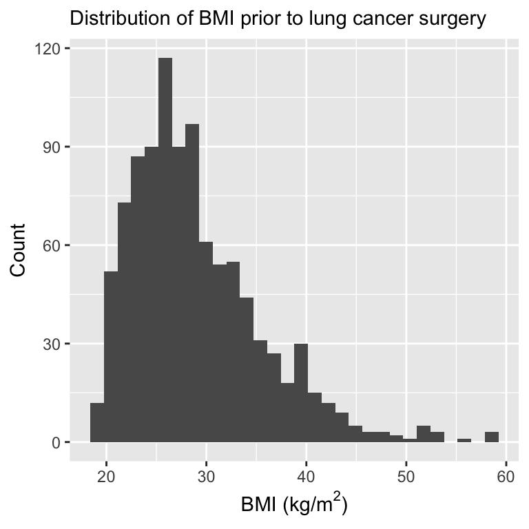
Researchers are interested in the association between the predictors: sex, marital status, and smoking history, and the outcome: BMI. They start by visualizing the distribution of BMI and notice that it is a bit right-skewed; and thus they are worried about performing linear regression. Instead they would like to perform median regression.
Setup a multivariable median regression model to estimate the association between the predictors: sex, marital status, and smoking history, and the outcome: BMI. Define the random variable \(Y_i\) as the BMI in \(kg/m^2\) for patient \(i\) and the median quantile of \(Y_i\) given predictors \(\mathbf{x}_i\) as \(q({Y_i|\mathbf{x}_i})\). We will model the median quantile as a linear function of the predictors, \[q({Y_i|\mathbf{x}_i}) = \alpha + \mathbf{x}_i\boldsymbol{\beta},\] where \(\mathbf{x}_i = (Male_i, Married_i, Current\_Smoker_i, Former\_Smoker_i).\) Each of these predictors is just a binary variable.
Exercise 1
Formulate this regression problem within the framework of a Bayesian model (hint: Laplace distribution!). Fit this regression using Stan to estimate \((\alpha, \boldsymbol{\beta})\) and any other parameters that arise in the model. For all model parameters, choose weakly-informative priors. Evaluate model convergence.
Exercise 2
Perform a posterior predictive check using the median as a test statistic. Be sure to present a posterior predictive p-value and use it to describe the model fit.
Exercise 3
Perform a posterior predictive check for the 2.5th and 97.5th quantiles. Comment on the difference between the result from Exercise 2.
Exercise 4
Present posterior summaries for all population parameters. For all predictors with a significant association (i.e., 95% credible interval does not include zero), provide an interpretation within the context of the problem.
Exercise 5
Fit the same model as in Exercise 1 using linear regression. Compare the posterior mean estimates of \(\boldsymbol{\beta}\) between the two models. Do they correspond?
Exercise 6
Perform a model comparison between the models in Exercise 1 and Exercise 5. Which model is preferred? Provide intuition for why one model may be preferred over the other.
Exercises 7-11
Define a binary outcome variable \(Y_i = 1(LengthofStay_i > 5)\) for \(i = 1,\ldots,n\). We are interested in performing logistic regression such that \(Y_i \stackrel{ind}{\sim}\text{Bernoulli}(\pi_i)\), where
\[\begin{align*} \text{logit} (\pi_i) &= \alpha + \beta_1 Age_i + \beta_2 Married_i + \beta_3 Yes\_Family\_History_i\\ &\hspace{1cm}+ \beta_4 Current\_Smoker_i + \beta_5 Former\_Smoker_i + \beta_6 Male_i\\ &\hspace{1cm}+ \beta_7 Cancer\_Stage2_i + \beta_8 Cancer\_Stage3_i + \beta_9 Cancer\_Stage4_i\\ &\hspace{1cm}+ \gamma_1 WBC_i + \gamma_2 RBC_i + \gamma_3 BMI_i + \gamma_4 IL6_i + \gamma_5 CRP_i\\ &= \alpha + \mathbf{x}_i \boldsymbol{\beta} + \mathbf{z}_i \boldsymbol{\gamma}. \end{align*}\]
The population parameters are \((\alpha, \boldsymbol{\beta},\boldsymbol{\gamma})\), where \(\boldsymbol{\beta} = (\beta_1, \ldots, \beta_9)\) and \(\boldsymbol{\gamma} = (\gamma_1,\ldots,\gamma_5)\). Use the following priors for the centered intercept and regression parameters, \(\alpha \sim N(0, 3^2)\) and \(\beta_j \sim N(0, 3^2)\) for \(j = 1,\ldots,p\) (\(p=9\)). The researchers would like to place a horseshoe prior on each \(\gamma_l\), \(l=1,\ldots,q\) (\(q = 5\)).
The horseshoe prior for \(\gamma_l\) is given by, \[\begin{align*} \gamma_l | \lambda_l, \tau, c &\sim N\left(0, \tau^2 \lambda_l^2\right),\\ \lambda_l &\sim \mathcal C^+(0,1),\\ \tau &\sim \mathcal C^+(0,\tau_0^2). \end{align*}\]
Be sure to standardize these predictors prior to assigning a horseshoe prior.
Exercise 7
Before fitting the horseshoe regression, a realistic value of \(\tau_0\) must be determined. Compute a realistic value for \(\tau_0\) based on the effective number of non-zero coefficients. Researchers have a prior belief that the number of non-zero coefficients will be equal to 1 (i.e., \(q_0 = 1\)). When computing \(\tau_0\) be sure to provide a visual justification by plotting the effective number of non-zero coefficients for your choice of \(\tau_0\).
Exercise 8
Fit the logistic regression model using the horseshoe prior above. Present model convergence diagnostics and make a statement about whether the MCMC sampler has converged.
Exercise 9
Visualize the posterior distributions for the population parameters \((\alpha, \boldsymbol{\beta}, \boldsymbol{\gamma})\). \(\alpha\) is the intercept on the scale of the original data. Make a statement about the impact of the horseshoe prior on the posterior shape for \(\boldsymbol{\gamma}\).
Exercise 10
Present posterior summaries for \((\alpha, \boldsymbol{\beta}, \boldsymbol{\gamma})\). Choose one predictor that is significant and provide an interpretation of the posterior mean.
Exercise 11
Visualize the posterior distribution of \(\pi_2\) and \(\pi_4\), which are the probability of having a length of stay greater than 5 days for observation \(Y_2\) and \(Y_4\), respectively (i.e., the second and fourth rows of the hdp dataset). Compute \(P(\pi_4 > \pi_2 | \mathbf{Y})\) and make a statement about which patient is more likely to have a longer length of stay.
Submission
You will submit the PDF documents for homeworks, and exams in to Gradescope as part of your final submission.
Warning
Before you wrap up the assignment, make sure all documents are updated on your GitHub repo. We will be checking these to make sure you have been practicing how to commit and push changes.
Remember – you must turn in a PDF file to the Gradescope page before the submission deadline for full credit.
To submit your assignment:
Access Gradescope through the menu on the BIOSTAT 725 Canvas site.
Click on the assignment, and you’ll be prompted to submit it.
Mark the pages associated with each exercise. All of the pages of your homework should be associated with at least one question (i.e., should be “checked”).
Grading
| Component | Points |
|---|---|
| Ex 1 | 8 |
| Ex 2 | 4 |
| Ex 3 | 5 |
| Ex 4 | 4 |
| Ex 5 | 4 |
| Ex 6 | 5 |
| Ex 7 | 3 |
| Ex 8 | 8 |
| Ex 9 | 3 |
| Ex 10 | 3 |
| Ex 11 | 3 |