AE 02: Posterior estimation using Gibbs sampling

Glaucoma disease progression

Published

January 16, 2025

Due date

Application exercises (AEs) are submitted by pushing your work to the relevant GitHub repo. AEs from Tuesday lectures should be submitted by Friday by 11:59pm ET, and AEs from Thursday lectures should be submitted by Sunday at 11:59pm ET. Because AEs are intended for in-class activities, there are no extensions given on AEs.

This AE is a demonstration and you do not have to turn anything in!

Final .qmd and .pdf files pushed to your GitHub repo
Note: For homeworks and exams, you will also be required to submit your final .pdf file submitted on Gradescope

Introduction

This AE will again demonstrate the process of using Github and RStudio to retrieve and complete assignments in this course. We will also continue looking at the glaucoma dataset and study a regression problem using Bayesian inference.

Learning goals

By the end of the AE, you will…

Be familiar with the workflow using RStudio and GitHub
Gain practice writing a reproducible report using Quarto
Practice version control using GitHub
Perform Gibbs sampling for Bayesian linear regression and compute some basic summaries

Getting Started

Clone the repo & start new RStudio project

Go to the course organization at github.com/biostat725-sp25 organization on GitHub.
Click on the repo with the prefix ae-02-. It contains the starter documents you need to complete the AE.
Click on the green CODE button, select Use SSH (this might already be selected by default, and if it is, you’ll see the text Clone with SSH). Click on the clipboard icon to copy the repo URL.
- See the HW 00 instructions if you have not set up the SSH key or configured git.
In RStudio, go to File $\to$ New Project $\to$ Version Control $\to$ Git.
Copy and paste the URL of your assignment repo into the dialog box Repository URL. Again, please make sure to have SSH highlighted under Clone when you copy the address.
Click Create Project, and the files from your GitHub repo will be displayed in the Files pane in RStudio.
Click AE 02.qmd to open the template Quarto file. This is where you will write up your code and narrative for the AE.

R packages

We will begin by loading R packages that we will use in this AE.

library(tidyverse)    # data wrangling and visualization
library(knitr)        # format output
library(mvtnorm)      # multivariate normal rng

Data

The data are on patients with glaucoma from the Rotterdam Ophthalmic Data Repository. Glaucoma is the leading cause of irreversible blindness world wide with over 60 million glaucoma patients as of 2012. Since impairment caused by glaucoma is irreversible, early detection of disease progression is crucial for effective treatment. Patients with glaucoma are routinely followed up and administered visual fields, a functional assessment of their vision. After each visual field test their current disease status is reported as a mean deviation value, measured in decibels (dB). A lower mean deviation indicates worse vision. An important predictor of disease progression is intraocular pressure (IOP), the pressure of fluids inside your eye.

We will focus on two variables:

iop: intraocular pressure, measured in millimeters of mercury (mmHg)
progression: rate of disease progression, measured as the number dB lost per year (dB/year)

The goal of this analysis is to use the IOP to understand variability in disease progression in glaucoma patients. The data is available in the ae-02- repo and is called glaucoma.rds.

glaucoma <- readRDS(file = "glaucoma.rds")
glimpse(glaucoma)

Rows: 139
Columns: 7
$ id          <int> 1, 2, 3, 4, 5, 6, 7, 8, 9, 10, 11, 12, 13, 14, 15, 16, 17,…
$ age         <dbl> 51.55616, 76.78356, 46.38356, 42.56712, 68.36438, 56.61644…
$ sex         <chr> "F", "F", "F", "M", "F", "F", "F", "F", "M", "M", "M", "M"…
$ iop         <dbl> 10.333333, 11.750000, 14.666667, 5.333333, 12.666667, 18.3…
$ baseline_md <dbl> -7.69, -5.38, -22.05, -13.99, -13.02, -7.13, -2.69, -9.43,…
$ severity    <chr> "Moderate", "Mild", "Severe", "Severe", "Severe", "Moderat…
$ progression <dbl> -0.190141797, -0.055098961, 0.431682497, 0.218545250, 0.08…

Exploratory data analysis

Let’s begin by examining the univariate distributions of the disease progression and IOP. The code to visualize and calculate summary statistics for progression is below.

ggplot(data = glaucoma, aes(x = progression)) + 
  geom_histogram() +
  labs(x = "Disease progression (db/year)", 
       y = "Count",
       title = "Disease progression in glaucoma patients")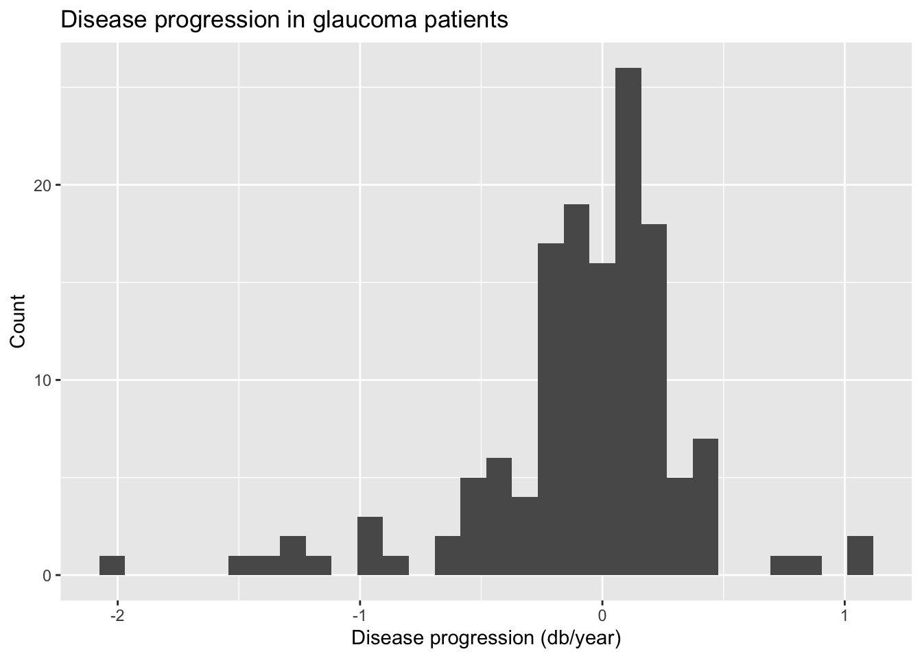

glaucoma |>
  summarise(min = min(progression), q1 = quantile(progression, 0.25), 
            median = median(progression), q3 = quantile(progression, 0.75), 
            max = max(progression), mean = mean(progression), sd = sd(progression)) |>
  kable(digits = 3)

min	q1	median	q3	max	mean	sd
-1.981	-0.207	-0.022	0.149	1.107	-0.079	0.441

Posterior estimation

You want to fit a model of the form

$p r o g r e s s i o n_{i} = β_{0} + β_{1} i o p_{i} + ϵ, ϵ \sim N (0, σ^{2}) .$

We can obtain samples from the posterior distribution for the regression parameters using the specification from the slides. We define the data objects needed for posterior estimation.

X <- cbind(1, glaucoma$iop) # covariate matrix
Y <- glaucoma$progression # outcome definition
p <- ncol(X) - 1 # number of covariates (excluding the intercept)
n <- length(Y) # number of observations

We will then define hyperparameters for the priors. We will choose a weakly informative prior. We will discuss more about priors in subsequent lectures. For now, we will place the following priors: $β \sim N (β_{0}, σ_{β}^{2} I_{2})$ and $σ^{2} \sim Inv-Gamma (a, b)$ .

sigma_beta2 <- 10
beta0 <- rep(0, p + 1)
a <- 3 
b <- 1

We can now obtain samples from the posterior using Gibbs sampling. Let’s set $S = 5, 000$ . We begin by randomly initializing $σ^{2}$ .

S <- 5000
sigma2 <- exp(rnorm(1)) # initial value

Run a for loop over samples.

samples <- NULL
for (s in 1:S) {
  
  ###Sample from full conditional for beta
  var_beta <- chol2inv(chol(t(X) %*% X / sigma2 + diag(p + 1) / sigma_beta2))
  mean_beta <- var_beta %*% (beta0 / sigma_beta2 + t(X) %*% Y / sigma2)
  beta <- as.numeric(rmvnorm(1, mean_beta, var_beta))
  
  ###Sample from full conditional for sigma2
  quadratic <- as.numeric(t(Y - X %*% beta) %*% (Y - X %*% beta))
  sigma2 <- 1 / rgamma(1, shape = a + n / 2, rate = b + quadratic / 2)
  
  ###Save samples
  samples <- rbind(samples, c(beta, sigma2))
  
}

Insepction of Gibbs sampler

We can begin by inspecting the posterior density and traceplots.

dat.fig <- data.frame(
  parameter = rep(c("beta[0]", "beta[1]", "sigma^2"), each = S),
  index = rep(1:S, 3),
  value = as.numeric(samples)
)
ggplot(dat.fig, aes(x = value)) +
  geom_density(lwd = 1.5) +
  facet_grid(. ~ parameter, labeller = label_parsed, scales = "free_x") +
  ylab("Density") +
  xlab("Parameter value")
ggplot(dat.fig, aes(x = index, y = value)) + 
  geom_line(lwd = 0.5) + 
  facet_grid(. ~ parameter, labeller = label_parsed, scales = "free_x") + 
  ylab("Parameter value") +
  xlab("Sample index")

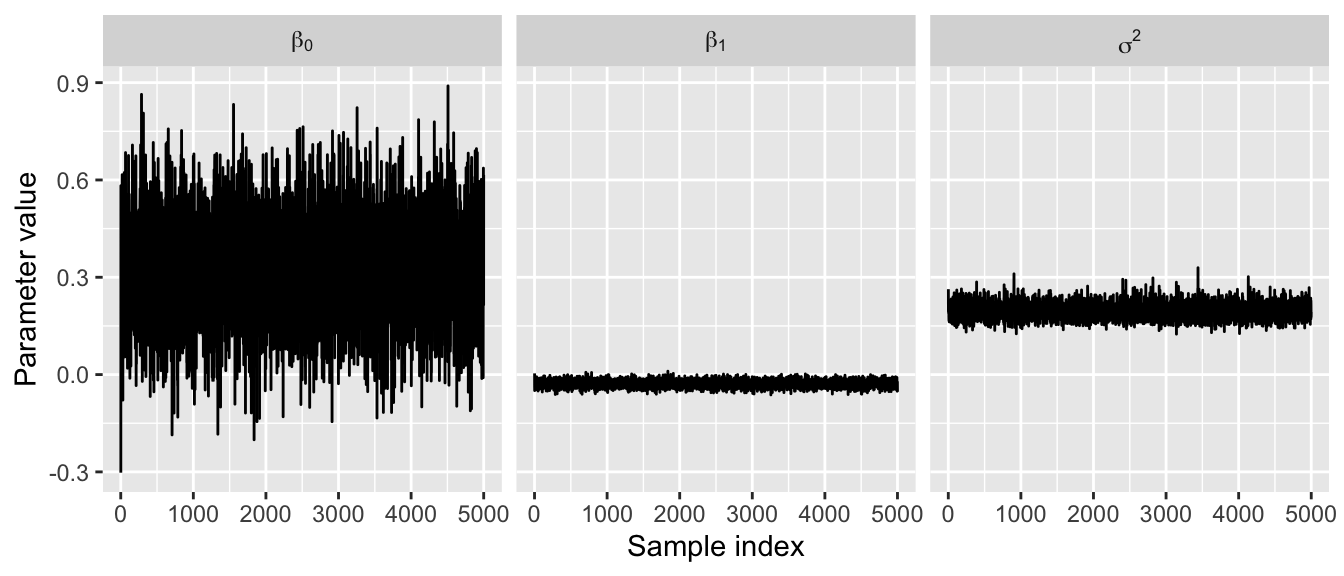
The traceplots do not exhibit much autocorrelation, indicating our samples have properly converged. We will dive into this much more in subsequent lectures.

Exercises

Exercise 1

Compute the posterior mean and standard deviation for the intercept, slope, and measurement error. Provide an interpretation for each of these parameter estimates.

Answer:

# add code here

Exercise 2

Compute a 95% confidence interval for the regression slope. Provide an interpretation for this confidence interval.

Answer:

# add code here

Exercise 3

Compute a one-sided Bayesian p-value for the regression slope: $P (β_{1} < 0)$ . Interpret the results in plain English. Is intraocular pressure associated with disease progression?

Answer:

# add code here

Important

To submit the AE:

Render the document to produce the PDF with all of your work from today’s class.
Push all your work to your AE repo on GitHub. You’re done! 🎉

This AE is a demonstration and you do not have to turn anything in!