library(tidyverse)     # data wrangling and visualization
library(knitr)         # format output
library(rstan)         # Stan
library(bayesplot)     # figures for post Stan inference
# new packages are below
library(sf)            # functions to work with spatial data
library(rnaturalearth) # maps of DRC
library(geodist) # conversion from geodisic to milesAE 09: Scalable Gaussian processes
Hilbert space methods for Gaussian process regression
Due date
Application exercises (AEs) are submitted by pushing your work to the relevant GitHub repo. AEs from Tuesday lectures should be submitted by Friday by 11:59pm ET, and AEs from Thursday lectures should be submitted by Sunday at 11:59pm ET. Because AEs are intended for in-class activities, there are no extensions given on AEs.
- Final
.qmdand.pdffiles pushed to your GitHub repo - Note: For homeworks and exams, you will also be required to submit your final
.pdffile submitted on Gradescope
Introduction
This AE will take another look at the hemoglobin dataset. We will use the Hilbert space methods for Gaussian processes (HSGP) to do a geospatial analysis on the full dataset.
Learning goals
By the end of the AE, you will…
- Learn how to implement HSGP with
Randstan - Analyze Bayesian geospatial modeling fitting results
Getting Started
Clone the repo & start new RStudio project
- Go to the course organization at github.com/biostat725-sp25 organization on GitHub.
- Click on the repo with the prefix ae-09-. It contains the starter documents you need to complete the AE.
- Click on the green CODE button, select Use SSH (this might already be selected by default, and if it is, you’ll see the text Clone with SSH). Click on the clipboard icon to copy the repo URL.
- See the HW 00 instructions if you have not set up the SSH key or configured git.
- In RStudio, go to File \(\rightarrow\) New Project \(\rightarrow\) Version Control \(\rightarrow\) Git.
- Copy and paste the URL of your assignment repo into the dialog box Repository URL. Again, please make sure to have SSH highlighted under Clone when you copy the address.
- Click Create Project, and the files from your GitHub repo will be displayed in the Files pane in RStudio.
- Click
ae-09.qmdto open the template Quarto file. This is where you will write up your code and narrative for the AE.
R packages
We will begin by loading R packages that we will use in this AE.
Data
Democratic Republic of Congo Demographic and Health Survey
We continue working on the hemoglobin dataset, with a sample of women aged 15-49 sampled from the 2013-14 Democratic Republic of Congo (DRC) Demographic and Health Survey. There are ~8600 women who are nested in ~500 survey clusters. The variables in the dataset are as follows.
loc_id: location id (i.e. survey cluster).hemoglobin: hemoglobin level (g/dL).anemia: anemia classifications.age: age in years.urban: urban vs. rural.LATNUM: latitude.LONGNUM: longitude.mean_hemoglobin: average hemoglobin at each community (g/dL).community_size: number of participants at each community.mean_age: average age of participants at each community (years).
The data set is available in your AE repos and is called drc.
data <- readRDS("drc.rds")Handling Spatial Data in R for HSGP
Center the coordinates
We first center the coordinates. In real applications, we might want to consider more sophisticated methods to properly transform longitude and latitude to Euclidean coordinates, but here we directly use them as Euclidean coordinates for simplicity.
### center coordinates
x_range <- round(range(data$LONGNUM),2)
y_range <- c(-13,5)

# center the locations
data_loc_centered <- data %>%
  mutate(LONGNUM = (LONGNUM - mean(x_range)),
         LATNUM = (LATNUM - mean(y_range)))

# extract unique locations
u <- data_loc_centered %>%
  filter(!duplicated(cbind(LONGNUM,LATNUM))) %>%
  dplyr::select(LONGNUM,LATNUM)
Obtain a Grid for Prediction
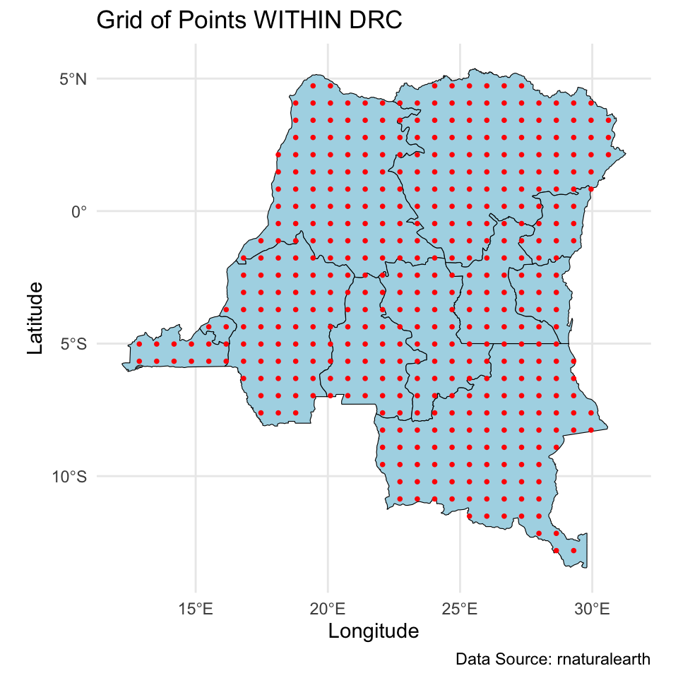
Next, we obtain locations for prediction. We first create a \(30 \times 30\) grid over DRC, and then extract points that are within DRC. This leaves us with about ~440 new locations. Remember to center these coordinates as well!
congo_states_map <- ne_states(country = "Democratic Republic of the Congo", returnclass = "sf")
congo_states_map <- st_transform(congo_states_map, crs = 4326)
bbox <- st_bbox(congo_states_map)

latitudes <- seq(bbox["ymin"], bbox["ymax"], length.out = 30)
longitudes <- seq(bbox["xmin"], bbox["xmax"], length.out = 30)
grid_points <- expand.grid(lat = latitudes, long = longitudes)

# Convert the grid into an sf object
grid_sf <- st_as_sf(grid_points, coords = c("long", "lat"), crs = 4326)
in_drc <- st_within(grid_sf, congo_states_map, sparse = FALSE)
in_drc <- apply(in_drc,1,any)

grid_inside_drc <- grid_sf[in_drc, ]

u_new <- st_coordinates(grid_inside_drc)

u_new[,1] <- (u_new[,1] - mean(x_range))
u_new[,2] <- (u_new[,2] - mean(y_range))
# Plot all the grid points
ggplot() +
geom_sf(data = congo_states_map, fill = "lightblue", color = "black") +
geom_sf(data = grid_sf, color = "red", shape = 16, size = 1) +
theme_minimal() +
labs(title = "Grid of Points across DRC",
caption = "",
# subtitle = "Red points represent valid grid points inside DRC boundaries",
x = "Longitude", y = "Latitude")
# Plot the grid points within the states
ggplot() +
geom_sf(data = congo_states_map, fill = "lightblue", color = "black") +
geom_sf(data = grid_inside_drc, color = "red", shape = 16, size = 1) +
theme_minimal() +
labs(title = "Grid of Points WITHIN DRC",
caption = "Data Source: rnaturalearth",
# subtitle = "Red points represent valid grid points inside DRC boundaries",
x = "Longitude", y = "Latitude")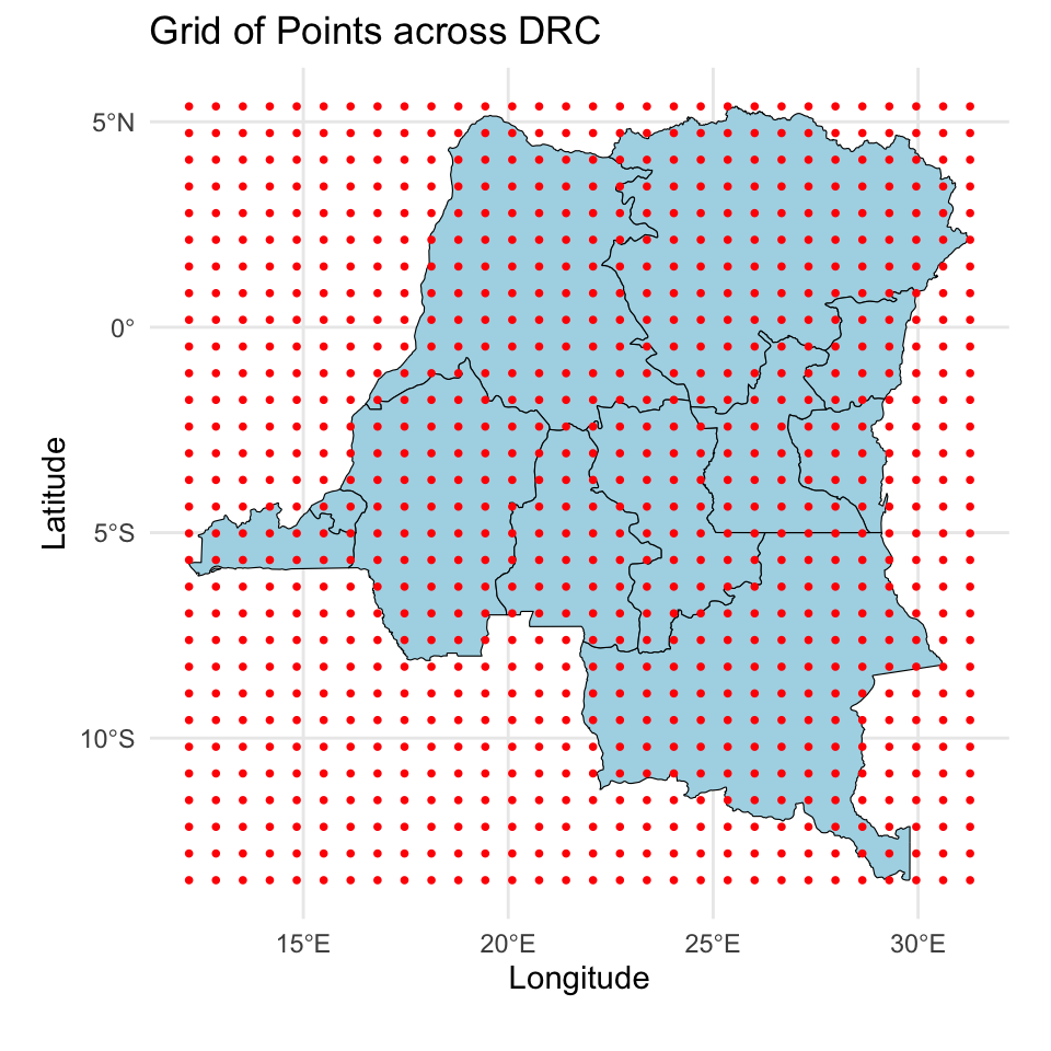
HSGP model fitting
We obtain the design matrix \(\mathbf{X}\) and the mapping table. Make sure \(\mathbf{X}\) doesn’t contain an intercept as that will be modeled separately through the \(\alpha\) parameter.
X <- model.matrix(~I(age/10)+urban,data=data)[,-1]
Ids <- match(
  paste(data_loc_centered$LONGNUM,data_loc_centered$LATNUM),
  paste(u$LONGNUM,u$LATNUM)
)
Compile the stan model.
mod <- stan_model(file = "22-hsgp-model.stan")Set stan run parameters and initialize parameter values for HSGP. Here we set \(\mathbf{S}\) to \((9.5,9)\) after checking the range of the centered coordinates. And we set the initial value of \(\rho\) to 5 which is in between half to one times the observed data box size as per recommendations in Riutort-Mayol et al.
range(data_loc_centered$LONGNUM)[1] -9.322493 9.324712range(data_loc_centered$LATNUM)[1] -8.607145 8.957885runspec <- list(maxiter=30,nburn=1000,niter=5000,nthin=5,nchains=4,
S=c(9.5,9),Y=data$hemoglobin,u=u,u_new=u_new,X=X,
Ids=Ids,rho0=5)Load HSGP helper functions and do a test run to make sure you can successfully run these codes. We only do 100 iterations for the test run so it should be quick. Later you can delete testshort=T to do the full run. These codes run 4 parallel chains, so make sure you run them on a suitable environment. It should take about 15-20 minutes.
source("functions.R")

j <- 1
runspec <- updateHSGP(runspec,j)

while (!runspec$check[[j]] & j<=runspec$maxiter){

  runspec <- runHSGP(runspec,mod,j,seed=j,testshort=T)
  j <- j+1
  runspec <- updateHSGP(runspec,j)

}
Save the model fitting results of the very last run for analysis. The stan fit object is saved in the list element named “fit”.
runspec$fit <- runspec$fit[[j-1]]
saveRDS(runspec,"res_HSGP.rds")
Exercise
Do a full HSGP run, and use the model fitting results to answer the following questions.
Exercise 1
How many iterations did HSGP parameter tuning process take? How many basis functions were used in the final HSGP run?
Answer:
# add code hereExercise 2
Look at the traceplots for a few parameters and comment on the mixing of the MCMC chain.
Answer:
# add code hereExercise 3
Obtain posterior mean and 95% credible interval for the regression coefficients. Interpret them under our context. Are age and urbanicity significantly associated with female hemoglobin level?
Answer:
# add code hereExercise 4
Use codes provided in the last AE to create visualizations of the surface of posterior mean and posterior SD of the spatial intercept. You can use the following codes to extract the posterior mean and SD. Note that due to the identifiability issue discussed in class, here we look at \(\alpha\mathbf{1}+\boldsymbol{\theta}^*\).
res_HSGP <- runspec$fit
p_theta_HSGP <- as.matrix(res_HSGP,pars="theta_new")
p_alpha_HSGP <- as.matrix(res_HSGP,pars="alpha")
p_intercept_HSGP <- p_theta_HSGP + c(p_alpha_HSGP)
p_intercept_HSGP_m <- colMeans(p_intercept_HSGP)
p_intercept_HSGP_sd <- apply(p_intercept_HSGP,2,sd)
Describe the spatial pattern of hemoglobin level for females in DRC, and think of possible reasons based on your knowledge about DRC.
Answer:
# add code here
Important
To submit the AE:
- Render the document to produce the PDF with all of your work from today’s class.
- Push all your work to your AE repo on GitHub. You’re done! 🎉