library(tidyverse)    # data wrangling and visualization
library(knitr)        # format output
library(rstan) # StanAE 03: Introduction to Stan
Modeling diabetes disease progression
Due date
Application exercises (AEs) are submitted by pushing your work to the relevant GitHub repo. AEs from Tuesday lectures should be submitted by Friday by 11:59pm ET, and AEs from Thursday lectures should be submitted by Sunday at 11:59pm ET. Because AEs are intended for in-class activities, there are no extensions given on AEs.
- Final
.qmdand.pdffiles pushed to your GitHub repo - Note: For homeworks and exams, you will also be required to submit your final
.pdffile submitted on Gradescope
Introduction
This AE will be an introduction to Stan using an example data set on diabetes disease progression. We will walk through a linear regression task using Stan and code up our first Stan model.
Learning goals
By the end of the AE, you will…
- Be familiar with the workflow using RStudio and GitHub
- Perform Bayesian linear regression using HMC
- Prepare data for a regression task in Stan
- Print posterior results from Stan
Getting Started
Clone the repo & start new RStudio project
- Go to the course organization at github.com/biostat725-sp25 organization on GitHub.
- Click on the repo with the prefix ae-03-. It contains the starter documents you need to complete the AE.
- Click on the green CODE button, select Use SSH (this might already be selected by default, and if it is, you’ll see the text Clone with SSH). Click on the clipboard icon to copy the repo URL.
- See the HW 00 instructions if you have not set up the SSH key or configured git.
- In RStudio, go to File \(\rightarrow\) New Project \(\rightarrow\) Version Control \(\rightarrow\) Git.
- Copy and paste the URL of your assignment repo into the dialog box Repository URL. Again, please make sure to have SSH highlighted under Clone when you copy the address.
- Click Create Project, and the files from your GitHub repo will be displayed in the Files pane in RStudio.
- Click
AE 03.qmdto open the template Quarto file. This is where you will write up your code and narrative for the AE.
R packages
We will begin by loading R packages that we will use in this AE.
Data
Today we will use data from the paper Least Angle Regression by Efron et al. There are ten baseline variables, age, sex, body mass index, average blood pressure, and six blood serum measurements were obtained for each of n = 442 diabetes patients, as well as the response of interest, a quantitative measure of disease progression one year after baseline.
We will focus on the following variables:
Y: measure of disease progression one year after baselineAGE: age in yearsSEX: sex (1= female,2= male)BMI: body mass index (\(kg/m^2\))BP: average blood pressure (mm Hg)
The goal of this analysis is to learn the associations between age, sex, BMI, and blood pressure on diabetic disease progression one year after baseline. The data is available in the ae-03- repo and is called diabetes.txt.
diabetes <- read_table("diabetes.txt")
glimpse(diabetes)
Rows: 442
Columns: 11
$ AGE <dbl> 59, 48, 72, 24, 50, 23, 36, 66, 60, 29, 22, 56, 53, 50, 61, 34, 47…
$ SEX <dbl> 2, 1, 2, 1, 1, 1, 2, 2, 2, 1, 1, 2, 1, 2, 1, 2, 1, 2, 1, 1, 1, 2, …
$ BMI <dbl> 32.1, 21.6, 30.5, 25.3, 23.0, 22.6, 22.0, 26.2, 32.1, 30.0, 18.6, …
$ BP <dbl> 101.00, 87.00, 93.00, 84.00, 101.00, 89.00, 90.00, 114.00, 83.00, …
$ S1 <dbl> 157, 183, 156, 198, 192, 139, 160, 255, 179, 180, 114, 184, 186, 1…
$ S2 <dbl> 93.2, 103.2, 93.6, 131.4, 125.4, 64.8, 99.6, 185.0, 119.4, 93.4, 5…
$ S3 <dbl> 38, 70, 41, 40, 52, 61, 50, 56, 42, 43, 46, 32, 62, 49, 72, 39, 70…
$ S4 <dbl> 4.00, 3.00, 4.00, 5.00, 4.00, 2.00, 3.00, 4.55, 4.00, 4.00, 2.00, …
$ S5 <dbl> 4.8598, 3.8918, 4.6728, 4.8903, 4.2905, 4.1897, 3.9512, 4.2485, 4.…
$ S6 <dbl> 87, 69, 85, 89, 80, 68, 82, 92, 94, 88, 83, 77, 81, 88, 73, 81, 98…
$ Y <dbl> 151, 75, 141, 206, 135, 97, 138, 63, 110, 310, 101, 69, 179, 185, …Exploratory data analysis
Let’s begin by examining the univariate distributions of the diabetes disease progression. The code to visualize and calculate summary statistics for Y is below.
ggplot(data = diabetes, aes(x = Y)) +
  geom_histogram() +
  labs(x = "Disease progression at one year from baseline",
       y = "Count",
       title = "Disease progression in diabetes patients")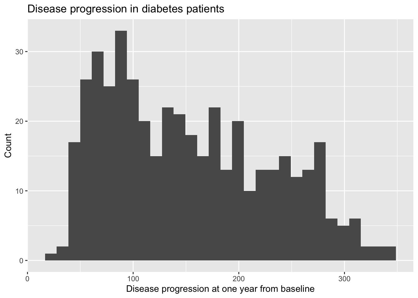
diabetes |>
  summarise(min = min(Y), q1 = quantile(Y, 0.25),
            median = median(Y), q3 = quantile(Y, 0.75),
            max = max(Y), mean = mean(Y), sd = sd(Y)) |>
kable(digits = 3)| min | q1 | median | q3 | max | mean | sd |
|---|---|---|---|---|---|---|
| 25 | 87 | 140.5 | 211.5 | 346 | 152.133 | 77.093 |
Exercises
Exercise 1
Fit the following model in Stan and present posterior summaries.
\[ Y_i = \alpha + \mathbf{x}_i\boldsymbol{\beta} + \epsilon_i, \hspace{5mm} \epsilon \sim N(0, \sigma^2), \] where \(\mathbf{x}_i = (Age_i, 1(Sex_i = Male), BMI_i, BP_i)\) and flat priors for all parameters: \(f(\alpha,\boldsymbol{\beta},\sigma) \propto c.\) Flat priors are specified by default, so we can omit any prior specification.
Answer:
# add code hereExercise 2
Fit the same model using the lm function in R. Compare the Bayesian and OLS/MLE results.
Answer:
# add code hereExercise 3
Fit the same regression model as in Exercise 1, but with the following priors:
\[\begin{align*} \alpha &\sim N(0,10)\\ \beta_j &\sim N(0,10),\quad j=1,\ldots,p\\ \sigma^2 &\sim \text{Inv-Gamma}(3,1). \end{align*}\]
Compare the results from this model to the previous two models.
Answer:
# add code here
Important
To submit the AE:
- Render the document to produce the PDF with all of your work from today’s class.
- Push all your work to your AE repo on GitHub. You’re done! 🎉