Bernoulli random variable: Used for binary outcomes (success/failure), e.g., whether a patient responds to a treatment (yes/no).
Binomial random variable: Used when there are multiple trials (e.g., 10 patients), and you want to model the number of successes (e.g., how many out of 10 patients experience a treatment response).
Bernoulli random variable example
A Bernoulli random variable represents a random variable with two possible outcomes: 0 or 1.
Scenario:
Imagine a medical study on a new drug for hypertension (high blood pressure). You want to model whether a patient responds positively to the treatment.
Success (1): The patient’s blood pressure decreases significantly (e.g., more than 10% reduction).
Failure (0): The patient does not experience a significant decrease in blood pressure.
Binomial random variable example
A Binomial random variable represents the number of successes in a fixed number of independent Bernoulli trials.
Scenario:
A clinical trial is conducted where 10 patients are given a new drug for diabetes. You want to model how many of these 10 patients experience a significant reduction in their blood sugar levels (e.g., a decrease by at least 20%).
Each patient’s outcome is a Bernoulli random variable: success (1) if their blood sugar level decreases, failure (0) if it does not.
The total number of successes (patients who experience a reduction) is modeled as a Binomial random variable.
Models for binary outcomes
Suppose \(Y_i \stackrel{ind}{\sim} \text{Bernoulli}(\pi_i)\) for \(i = 1,\ldots,n\). The pmf is,
The Mayo Clinic conducted a trial for primary biliary cirrhosis, comparing the drug D-penicillamine vs. placebo. Patients were followed for a specified duration, and their status at the end of follow-up (whether they died) was recorded.
Researchers are interested in predicting whether a patient died based on the following variables:
ascites: whether the patient had ascites (1 = yes, 0 = no)
bilirubin: serum bilirubin in mg/dL
stage: histologic stage of disease (ordinal categorical variable with stages 1, 2, 3, and 4)
Additionally, as a probability, \(P(Y_i = 1)\) must be in the interval [0, 1], but there is nothing in the model that enforces this constraint, so that you could be estimating probabilities that are negative or that are greater than 1!
From probabilities to log-odds
Suppose the probability of an event is \(\pi\).
Then the odds that the event occurs is \(\frac{\pi}{1 - \pi}\).
Taking the (natural) log of the odds, we have the logit of \(\pi\): the log-odds:
Note that although \(\pi\) is constrained to lie between 0 and 1, the logit of \(\pi\) is unconstrained - it can be anything from \(-\infty\) to \(\infty\).
Logistic regression model
Let’s create a model for the logit of \(\pi\): \(\text{logit}(\pi_i)= \eta_i\), where \(\eta_i = \alpha + \mathbf{x}_i \boldsymbol{\beta}.\)
This is a linear model for a transformation of the outcome of interest, and is also equivalent to,
The expression on the right is called a logistic function and cannot yield a value that is negative or a value that is >1. Fitting a model of this form is known as logistic regression.
Negative logits represent probabilities less than one-half.
\(\eta_i < 0 \implies \pi_i < 0.5\).
Positive logits represent probabilities greater than one-half.
\(\eta_i > 0 \implies \pi_i > 0.5\).
Interpreting parameters in logistic regression
Typically we interpret functions of parameters in logistic regression rather than the parameters themselves.
For the simple model: \(\log\left(\frac{\pi_i}{1 - \pi_i}\right) = \alpha + \beta X_{i},\) we note that the probability that \(Y_i = 1\) when \(X_i = 0\) is
Suppose that \(X\) is a binary (0/1) variable (e.g., \(X = 1\) for males and 0 for non-males).
In this case, we interpret \(\exp(\beta)\) as the odds ratio (OR) of the response for the two possible levels of \(X\).
For \(X\) on other scales, \(\exp(\beta)\) is interpreted as the odds ratio of the response comparing two values of \(X\) one unit apart.
Why?
Interpreting parameters in logistic regression
The log odds of response for \(X = 1\) is given by \(\alpha + \beta\), and the log odds of response for \(X = 0\) is \(\alpha\).
So the odds ratio of response comparing \(X = 1\) to \(X = 0\) is given by \(\frac{\exp(\alpha + \beta)}{\exp(\alpha)} = \exp(\beta)\).
In a multivariable logistic regression model with more than one predictor, this OR is interpreted conditionally on values of other variables (i.e., controlling for them).
Bayesian logistic regression
We start with observations \(Y_i \in \{0,1\}\) for \(i = 1,\ldots,n\), where \(Y_i \stackrel{ind}{\sim} \text{Bernoulli}(\pi_i)\), \(\pi_i = P(Y_i = 1)\).
The log-odds are modeled as \(\text{logit}(\pi_i) = \alpha + \mathbf{x}_i \boldsymbol{\beta} = \eta_i\).
To complete the Bayesian model specification, we must place priors on \(\alpha\) and \(\boldsymbol{\beta}\).
All priors we have discussed up-to-this point apply!
Historically, this was a difficult model to fit, but can be easily implemented in Stan.
Logistic regression in Stan
// Saved in logistic_regression.standata {int<lower = 1> n;int<lower = 1> p;int Y[n]; // Y is now type intmatrix[n, p] X;}transformed data {matrix[n, p] X_centered; // We are only centering X!row_vector[p] X_bar;for (i in1:p) { X_bar[i] = mean(X[, i]); X_centered[, i] = X[, i] - X_bar[i]; }}parameters {real alpha;vector[p] beta;}model {target += bernoulli_logit_lpmf(Y | alpha + X_centered * beta); // bernoulli likelihood parameterized in logitstarget += normal_lpdf(alpha | 0, 10);target += normal_lpdf(beta | 0, 10);}generated quantities {real pi_average = exp(alpha) / (1 + exp(alpha));vector[n] Y_pred;vector[n] log_lik;for (i in1:n) { Y_pred[i] = bernoulli_logit_rng(alpha + X_centered[i, ] * beta); log_lik[i] = bernoulli_logit_lpmf(Y[i] | alpha + X_centered[i, ] * beta); }}
library(rstan)compiled_model <-stan_model(file ="logistic_regression.stan")fit <-sampling(compiled_model, data = stan_data)print(fit, pars =c("alpha", "beta", "pi_average"), probs =c(0.025, 0.5, 0.975))
Inference for Stan model: anon_model.
4 chains, each with iter=2000; warmup=1000; thin=1;
post-warmup draws per chain=1000, total post-warmup draws=4000.

           mean se_mean   sd  2.5%  50% 97.5% n_eff Rhat
alpha      0.21    0.00 0.19 -0.14 0.20  0.60  1819 1.00
beta[1]    2.24    0.03 1.32  0.12 2.12  5.30  2328 1.00
beta[2]    0.38    0.00 0.08  0.24 0.38  0.55  2027 1.00
beta[3]    1.79    0.04 1.31 -0.43 1.65  4.86  1097 1.01
beta[4]    2.26    0.04 1.30  0.10 2.14  5.27  1073 1.01
beta[5]    2.69    0.04 1.31  0.52 2.54  5.74  1069 1.01
pi_average 0.55    0.00 0.05  0.47 0.55  0.65  1826 1.00

Samples were drawn using NUTS(diag_e) at Mon Feb 17 09:17:32 2025.
For each parameter, n_eff is a crude measure of effective sample size,
and Rhat is the potential scale reduction factor on split chains (at
convergence, Rhat=1).
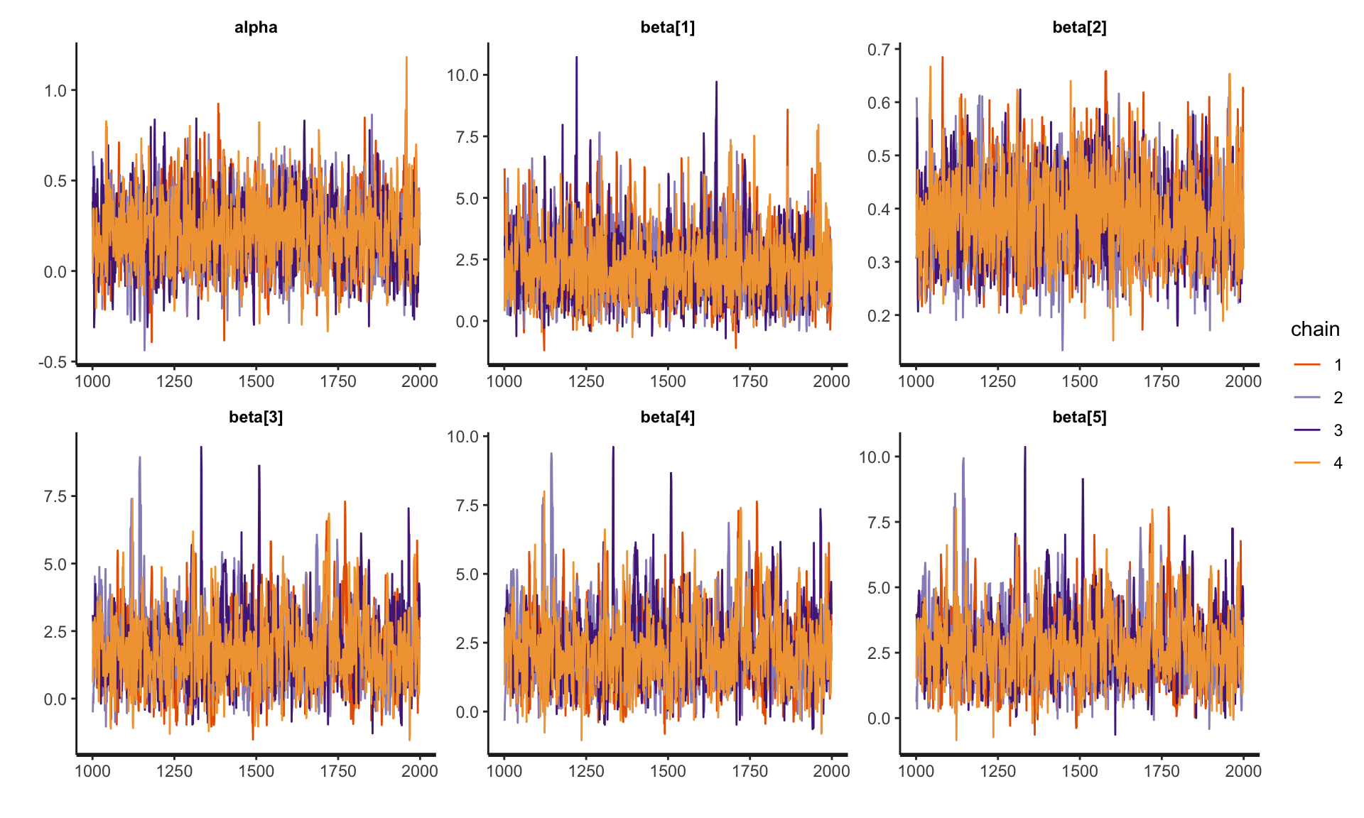
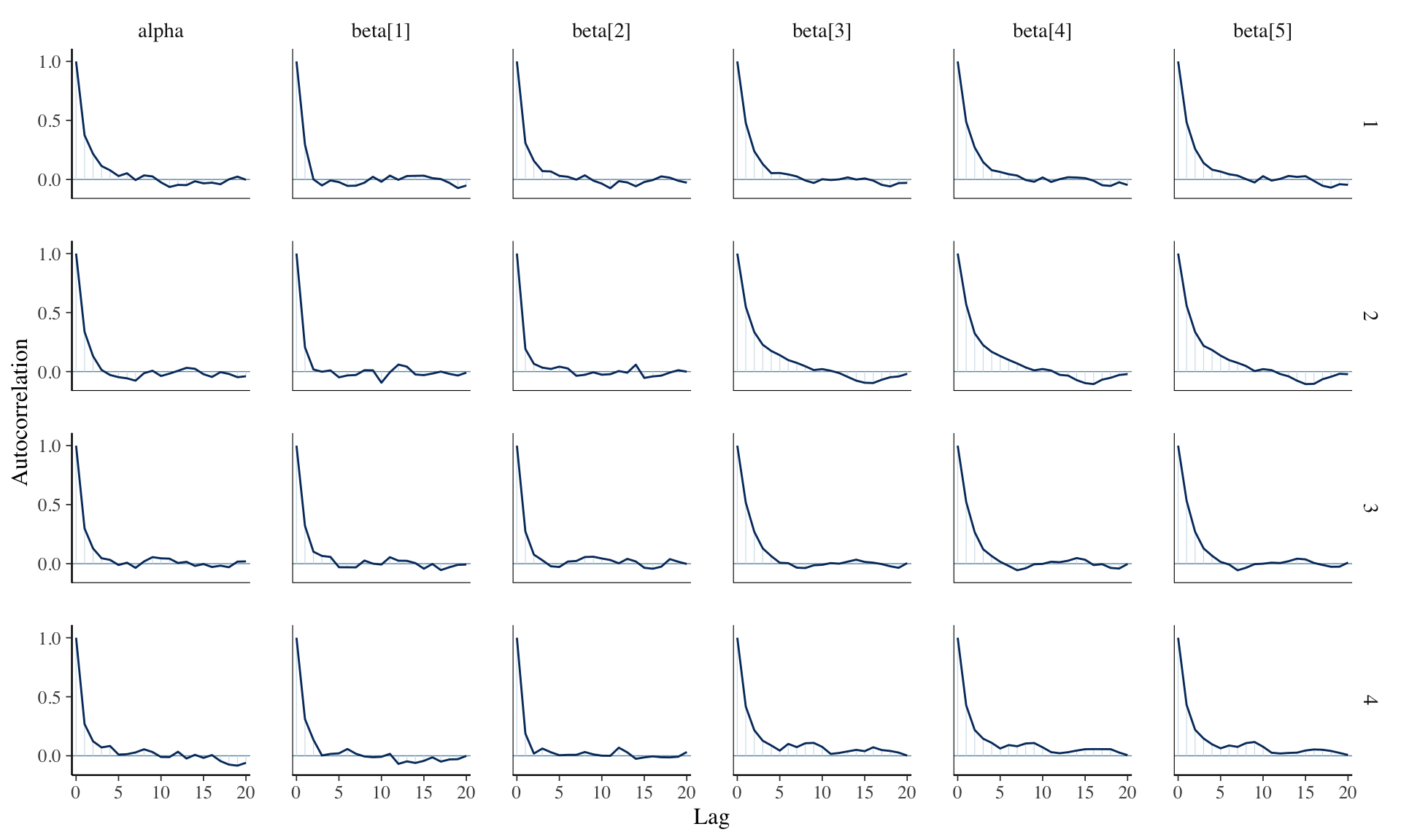
Convergence diagnostics
Convergence diagnostics
Back to the PBC data
Fitting a logistic regression model, we obtain
variable
mean
sd
2.5%
97.5%
alpha
intercept
0.21
0.00
-0.14
0.60
beta[1]
ascites
2.24
0.03
0.12
5.30
beta[2]
bilirubin
0.38
0.00
0.24
0.55
beta[3]
stage == 2
1.79
0.04
-0.43
4.86
beta[4]
stage == 3
2.26
0.04
0.10
5.27
beta[5]
stage == 4
2.69
0.04
0.52
5.74
How might we interpret these coefficients as odds ratios?
Back to the PBC data
Remember, we are interested in the probability that a patient died during follow-up (a “success”). We are predicting the log-odds of this event happening.
The posterior mean for ascites was 2.24. Thus, the odds ratio for dying is \(\exp(2.24) \approx 9.40\). That is, patients with ascites have 9 times the odds of dying compared to patients that do not, holding all other variables constant.
The posterior mean for bilirubin was 0.38. Thus, the odds ratio for dying for a patient with 1 additional mg/dL serum bilirubin compared to another is \(\exp(0.38) \approx 1.46\), holding all other variables constant.
The baseline stage was 1. The posterior mean for stage 3 was 2.26. Thus, patients in stage 3 have approximately 9.58 times the odds of dying compared to patients that do not, holding all other variables constant.
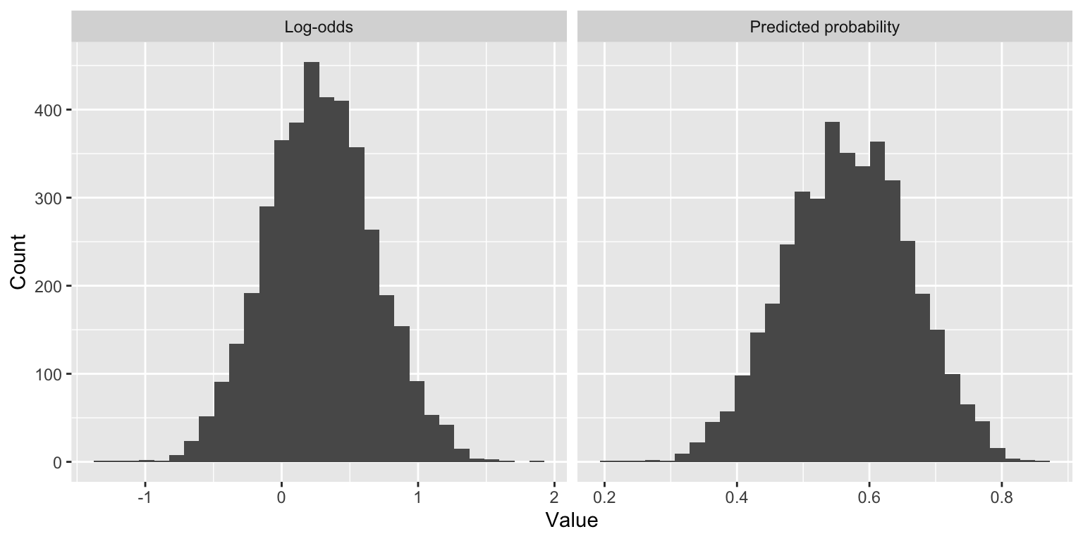
Predicted probabilities
There is a one-to-one relationship between \(\pi\) and \(\text{logit}(\pi)\). So, if we predict \(\text{logit}(\pi)\), we can “back-transform” to get back to a predicted probability.
For instance, suppose a patient does not have ascites, has a bilirubin level of 5 mg/dL, and is a stage 2 patient.
Inference for Stan model: anon_model.
4 chains, each with iter=2000; warmup=1000; thin=1;
post-warmup draws per chain=1000, total post-warmup draws=4000.

        mean se_mean   sd  2.5%  50% 97.5% n_eff Rhat
eta_new 0.28    0.01 0.40 -0.48 0.27  1.07  2754    1
pi_new  0.57    0.00 0.09  0.38 0.57  0.75  2780    1
Y_new   0.57    0.01 0.49  0.00 1.00  1.00  4013    1

Samples were drawn using NUTS(diag_e) at Mon Feb 17 09:17:32 2025.
For each parameter, n_eff is a crude measure of effective sample size,
and Rhat is the potential scale reduction factor on split chains (at
convergence, Rhat=1).
Predicted probabilities
Posterior mean of the predicted probabilities is 0.57.
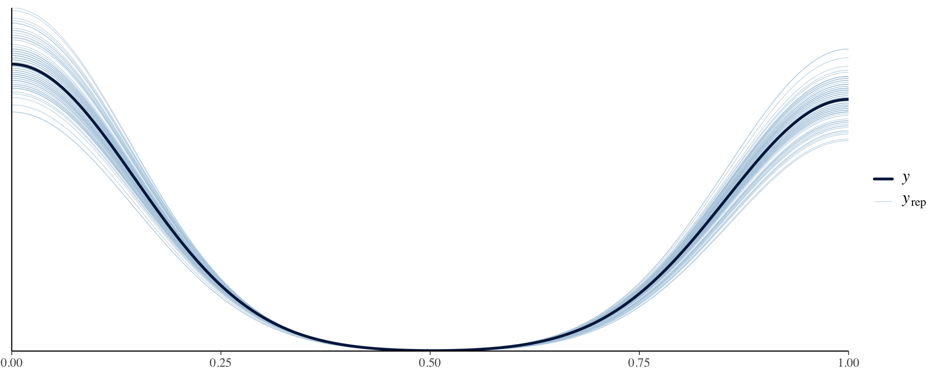
Posterior predictive checks
y_pred <- rstan::extract(fit, pars ="Y_pred")$Y_predppc_dens_overlay(stan_data$Y, y_pred[1:100, ])
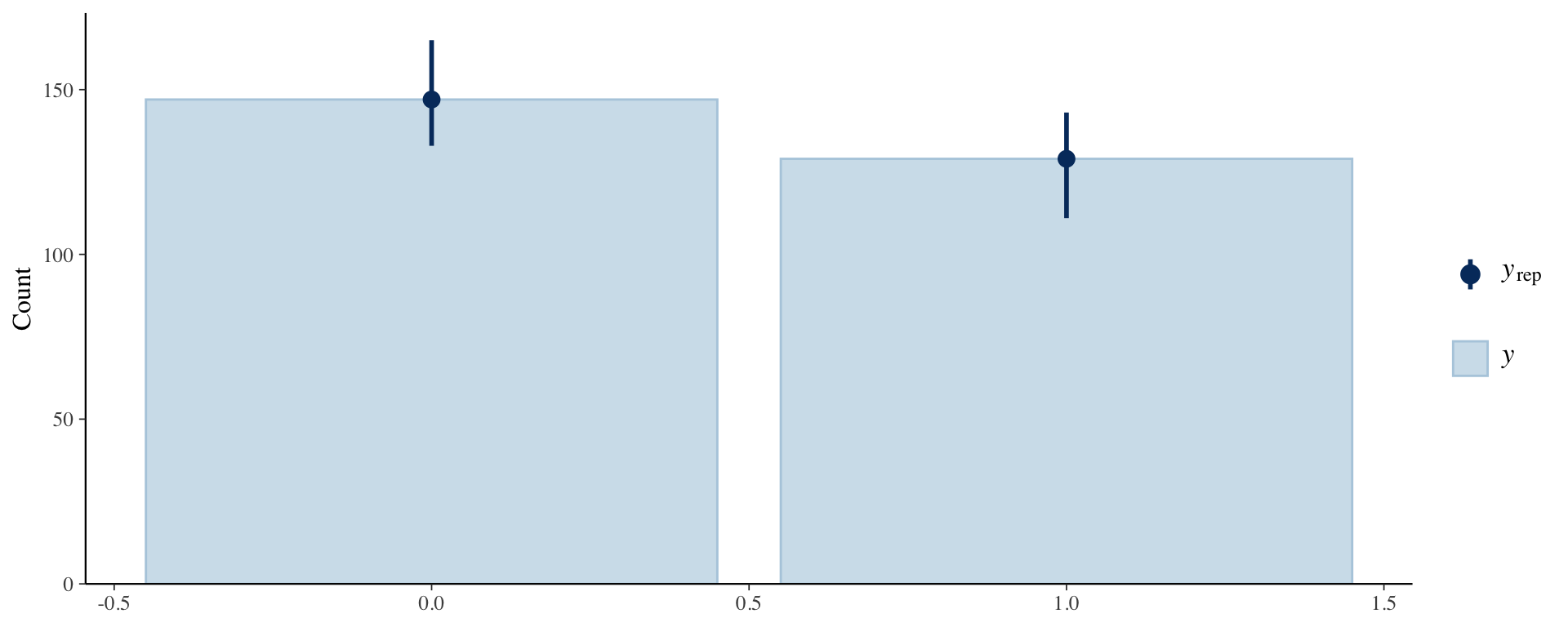
Posterior predictive checks
ppc_bars(stan_data$Y, y_pred[1:100, ])
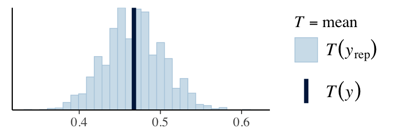
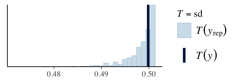
Posterior predictive checks
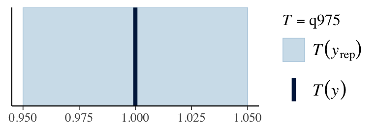
ppc_stat(stan_data$Y, y_pred, stat ="mean") # from bayesplotppc_stat(stan_data$Y, y_pred, stat ="sd")q025 <-function(y) quantile(y, 0.025)q975 <-function(y) quantile(y, 0.975)ppc_stat(stan_data$Y, y_pred, stat ="q025")ppc_stat(stan_data$Y, y_pred, stat ="q975")
Model comparison
Comparing our model to a baseline that removed stage.
An alternative approach is Probit regression, where we use the CDF of the standard normal distribution instead of the logit link: \(\Phi^{-1}(\pi) = \alpha + \beta X\)
Where \(\Phi^{-1}\) is the inverse normal CDF (also called the probit link function).
data {int<lower = 1> n; // number of observationsint<lower = 1> p; // number of predictorsint<lower = 0, upper = 1> Y[n]; // binary outcome (0 or 1)matrix[n, p] X; // design matrix (predictors)}parameters {real alpha; // interceptvector[p] beta; // coefficients}model {target += bernoulli_lpmf(Phi(alpha + X * beta)); // Probit model}
Steps to selecting a Bayesian GLM
Identify the support of the response distribution.
Select the likelihood by picking a parametric family of distributions with this support.
Choose a link function \(g\) that transforms the range of parameters to the whole real line.
Specify a linear model on the transformed parameters.