BIOSTAT 725 - Spring 2025 – Regularization

Review of last lecture

On Tuesday, we learned about robust regression.
- Heteroskedasticity
- Heavy-tailed distributions
- Median regression
These were all models for the observed data $Y_{i}$ .
Today, we will focus on prior specifications for $β$ .

Sparsity in regression problems

Supervised learning can be cast as the problem of estimating a set of coefficients $β = {β_{j}}_{j = 1}^{p}$ that determines some functional relationship between a set of ${x_{i j}}_{j = 1}^{p}$ and a target variable $Y_{i}$ .
This is a central focus of statistics and machine learning.
Challenges arise in “large- $p$ ” problems where, in order to avoid overly complex models that predict poorly, some form of dimension reduction is needed.
Finding a sparse solution, where some $β_{j}$ are zero, is desirable.

Bayesian sparse estimation

From a Bayesian-learning perspective, there are two main sparse-estimation alternatives: discrete mixtures and shrinkage priors.
Discrete mixtures have been very popular, with the spike-and-slab prior being the gold standard.
- Easy to force $β_{j}$ to exactly zero, but require discrete parameter specification.
Shrinkage priors force $β_{j}$ to zero using regularization, but struggle to get exact zeros.
- In recent years, shrinkage priors have become dominant in Bayesian sparsity priors.

Global-local shrinkage

Let’s assume $Y \overset{}{\sim} N (α + X β, σ^{2} I_{n})$ .
Sparsity can be induced into $β$ using a global-local prior,

$\begin{aligned} β_{j} | λ_{j}, τ & \overset{i n d}{\sim} N (0, λ_{j}^{2} τ^{2}) \\ λ_{j} & \overset{i i d}{\sim} f (λ_{j}) . \end{aligned}$

$τ^{2}$ is the global variance term.
$λ_{j}$ is the local term.
The degree of sparsity depends on the choice of $f (λ_{j})$ .

Spike-and-slab prior

Discrete parameter specification,

$\begin{aligned} β_{j} | λ_{j}, τ & \overset{i n d}{\sim} N (0, λ_{j}^{2} τ^{2}) \\ λ_{j} & \overset{i i d}{\sim} Bernoulli (π) . \end{aligned}$

$λ_{j} \in {0, 1}$ , thus this model permits exact zeros.
The number of zeros is dictated by $π$ , which can either be pre-specified or given a prior.
Discrete parameters can not be specified in Stan!

Spike-and-slab prior

Spike-and-slab can be written generally as a two-component mixture of Gaussians,

$\begin{aligned} β_{j} | λ_{j}, τ, ω & \overset{i n d}{\sim} λ_{j} N (0, τ^{2}) + (1 - λ_{j}) N (0, ω^{2}) \\ λ_{j} & \overset{i i d}{\sim} Bernoulli (π) . \end{aligned}$

$ω ≪ τ$ and the indicator variable $λ_{j} \in {0, 1}$ denotes whether $β_{j}$ is close to zero (comes from the “spike”, $λ_{j} = 0$ ) or non-zero (comes from the “slab”, $λ_{j} = 1$ ).
Often $ω = 0$ (the spike is a true spike).

Ridge regression

Ridge regression is motivated by extending linear regression to the setting where:
- there are too many predictors (sparsity is desired) and/or,
- $X^{⊤} X$ is ill-conditioned were singular or nearly singular (multicollinearity).
The OLS estimate becomes unstable: ${\hat{β}}_{OLS} = {(X^{⊤} X)}^{- 1} X^{⊤} Y .$

Ridge regression

The ridge estimator minimizes the penalized sum of squares,

${\hat{β}}_{RIDGE} = \arg min_{β} | | Y - μ | |_{2}^{2} + λ \sum_{j = 1}^{p} β_{j}^{2}$

$μ = α + X β$ .
$| | v | |_{2} = \sqrt{v^{⊤} v}$ is the L2 norm.
${\hat{β}}_{RIDGE} = {(X^{⊤} X + λ I_{p})}^{- 1} X^{⊤} Y$
- Adding the $λ$ to diagonals of $X^{⊤} X$ stabilizes the inverse, which becomes unstable with multicollinearity.

Bayesian ridge prior

Ridge regression can be obtained using the following global-local shrinkage prior,

$\begin{aligned} β_{j} | λ_{j}, τ & \overset{i n d}{\sim} N (0, λ_{j}^{2} τ^{2}) \\ λ_{j} & = 1 / λ \\ τ^{2} & = σ^{2} . \end{aligned}$

This is equivalent to: $f (β_{j} | λ, σ) \overset{i i d}{\sim} N (0, \frac{σ^{2}}{λ})$ .
How is this equivalent to ridge regression?

Bayesian ridge prior

The negative log-posterior is proportional to,

$\frac{| | Y - μ | |_{2}^{2}}{2 σ^{2}} + \frac{λ \sum_{j = 1}^{p} β_{j}^{2}}{2 σ^{2}} .$

The posterior mean and mode are ${\hat{β}}_{RIDGE}$ .
Since $λ$ is applied to the squared norm of the $β$ , people often standardize all of the covariates to make them have a similar scale.
Bayesian statistics is inherently performing regularization!

Lasso regression

The least absolute shrinkage and selection operator (lasso) estimator minimizes the penalized sum of squares,

${\hat{β}}_{LASSO} = \arg min_{β} | | Y - μ | |_{2}^{2} + λ \sum_{j = 1}^{p} | β_{j} |$

$λ = 0$ reduces to OLS etimator.
$λ = \infty$ leads to ${\hat{β}}_{LASSO} = 0$ .
Lasso is desirable because it can set some $β_{j}$ exactly to zero.

Bayesian lasso prior

Lasso regression can be obtained using the following global-local shrinkage prior,

$\begin{aligned} β_{j} | λ_{j}, τ & \overset{i n d}{\sim} N (0, λ_{j}^{2} τ^{2}) \\ λ_{j}^{2} & \overset{i i d}{\sim} Exponential (0.5) . \end{aligned}$

This is equivalent to: $f (β_{j} | τ) \overset{i i d}{\sim} Laplace (0, τ)$ .
How is this equivalent to lasso regression?

Bayesian lasso prior

The negative log-posterior is proportional to,

$\frac{| | Y - μ | |_{2}^{2}}{2 σ^{2}} + \frac{\sum_{j = 1}^{p} | β_{j} |}{τ} .$

Lasso is recovered by specifying: $λ = 1 / τ$ .
The posterior mode is ${\hat{β}}_{LASSO}$ .
As $λ$ increases, more coefficients are set to zero (less variables are selected), and among the non-zero coefficients, more shrinkage is employed.

Bayesian lasso does not work

There is a consensus that the Bayesian lasso does not work well.
It does not yield $β_{j}$ that are exactly zero and it can overly shrink non-zero $β_{j}$ .
The gold-standard sparsity-inducing prior in Bayesian statistics is the horseshoe prior.

Relevance vector machine

Before we get to the horseshoe, one more global-local prior, called the relevance vector machine.
This model can be obtained using the following prior,

$\begin{aligned} β_{j} | λ_{j}, τ & \overset{i n d}{\sim} N (0, λ_{j}^{2} τ^{2}) \\ λ_{j}^{2} & \overset{i i d}{\sim} Inverse-Gamma (\frac{ν}{2}, \frac{ν}{2}) . \end{aligned}$

This is equivalent to: $f (β_{j} | τ) \overset{i i d}{\sim} t_{ν} (0, τ)$ .

Horseshoe prior

The horseshoe prior is specified as,

$\begin{aligned} β_{j} | λ_{j}, τ & \overset{i n d}{\sim} N (0, λ_{j}^{2} τ^{2}) \\ λ_{j} & \overset{i i d}{\sim} C^{+} (0, 1), \end{aligned}$ where $C^{+} (0, 1)$ is a half-Cauchy distribution for the local parameter $λ_{j}$ .
- $λ_{j}$ ’s are the local shrinkage parameters.
- $τ$ is the global shrinkage parameter.

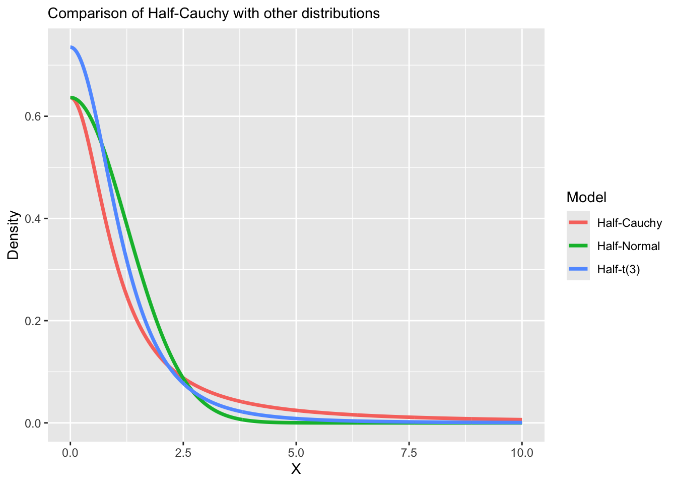
Half-Cauchy distribution

A random variable $X \sim C^{+} (μ, σ)$ follows a half-Cauchy distribution with location $μ$ and scale $σ > 0$ and has the following density,

$f (X | μ, σ) = \frac{2}{π σ} \frac{1}{1 + (X - μ)^{2} / σ^{2}}, X \geq μ$

The Half-Cauchy distribution with $μ = 0$ is a useful prior for non-negative parameters that may be very large, as allowed by the very heavy tails of the Cauchy distribution.

Half-Cauchy distribution in Stan

In Stan, the half-Cauchy distribution can be specified by putting a constraint on the parameter definition.

parameters {
  real<lower = 0> lambda;
}
model {
  target += cauchy_lpdf(lambda | 0, 1);
}

Half-Cauchy distribution

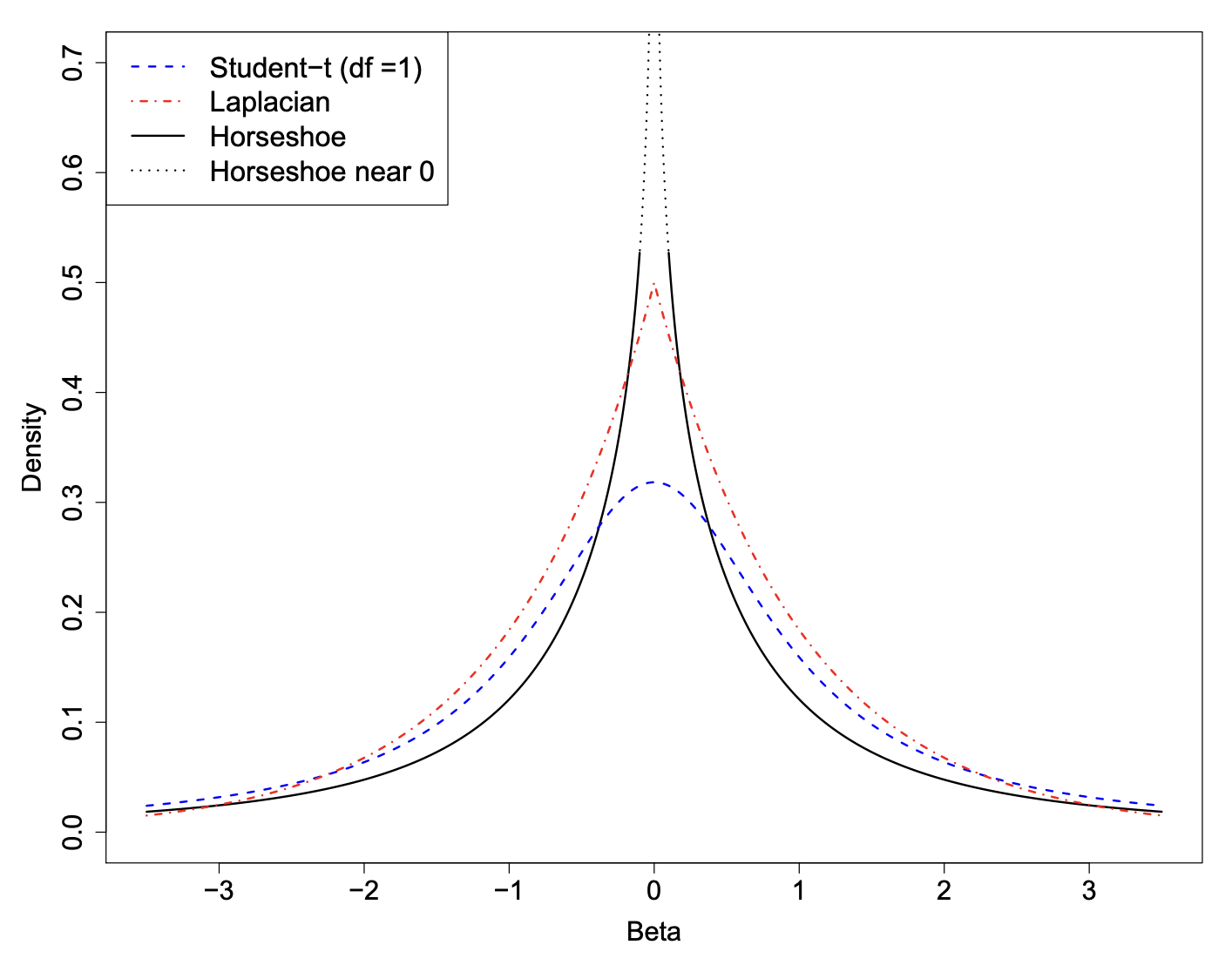
Horseshoe prior

The horseshoe prior has two interesting features that make it particularly useful as a shrinkage prior for sparse problems.

It has flat, Cauchy-like tails that allow strong signals to remain large (that is, un-shrunk) a posteriori.
It has an infinitely tall spike at the origin that provides severe shrinkage for the zero elements of $β$ .

As we will see, these are key elements that make the horseshoe an attractive choice for handling sparse vectors.

Relation to other shrinkage priors

$\begin{aligned} β_{j} | λ_{j}, τ & \sim N (0, λ_{j}^{2} τ^{2}) \\ λ_{j}^{2} & \sim f (λ_{j}) \end{aligned}$

$λ_{j} = 1 / λ$ , implies ridge regression.
$f (λ_{j}) = Exponential (0.5)$ , implies lasso.
$f (λ_{j}) = Inverse-Gamma (\frac{ν}{2}, \frac{ν}{2})$ , implies relevance vector machine.
$f (λ_{j}) = C^{+} (0, 1)$ , implies horseshoe.

Horsehoe density

workflow

From Carvalho 2009

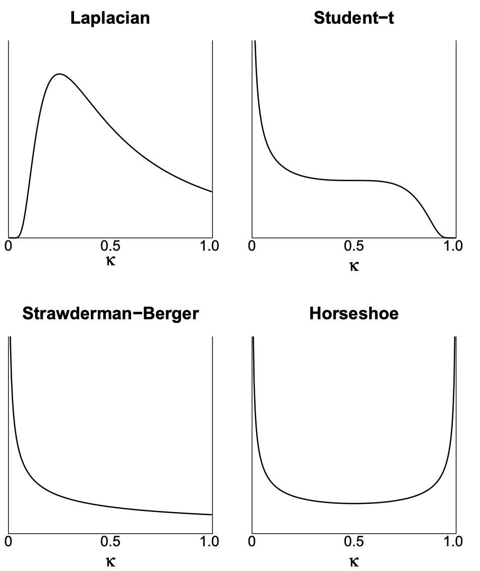
Shrinkage of each prior

Define the posterior mean of $β_{j}$ as ${\bar{β}}_{j}$ and the maximum likelihood estimator for $β_{j}$ as ${\hat{β}}_{j}$ .
The following relationship holds: ${\bar{β}}_{j} = (1 - κ_{j}) {\hat{β}}_{j}$ ,

$κ_{j} = \frac{1}{1 + n σ^{- 2} τ^{2} s_{j}^{2} λ_{j}^{2}} .$

$κ_{j}$ is called the shrinkage factor for $β_{j}$ .
$s_{j}^{2} = V (x_{j})$ is the variance for each predictor.

Standardization of predictors

In regularization problems, predictors are standardized (to mean zero and standard deviation one).
This means that so that $s_{j} = 1$ .
Shrinkage parameter:

$κ_{j} = \frac{1}{1 + n σ^{- 2} τ^{2} λ_{j}^{2}} .$

$κ_{j} = 1$ , implies complete shrinkage.
$κ_{j} = 0$ , implies no shrinkage.

Shrinkage parameter

workflow

From Carvalho 2009

Horseshoe shrinkage parameter

Choosing $λ_{j} \sim C^{+} (0, 1)$ implies $κ_{j} \sim Beta (0.5, 0.5)$ , a density that is symmetric and unbounded at both 0 and 1.
This horseshoe-shaped shrinkage profile expects to see two things a priori:
1. Strong signals ( $κ \approx 0$ , no shrinkage), and
2. Zeros ( $κ \approx 1$ , total shrinkage).

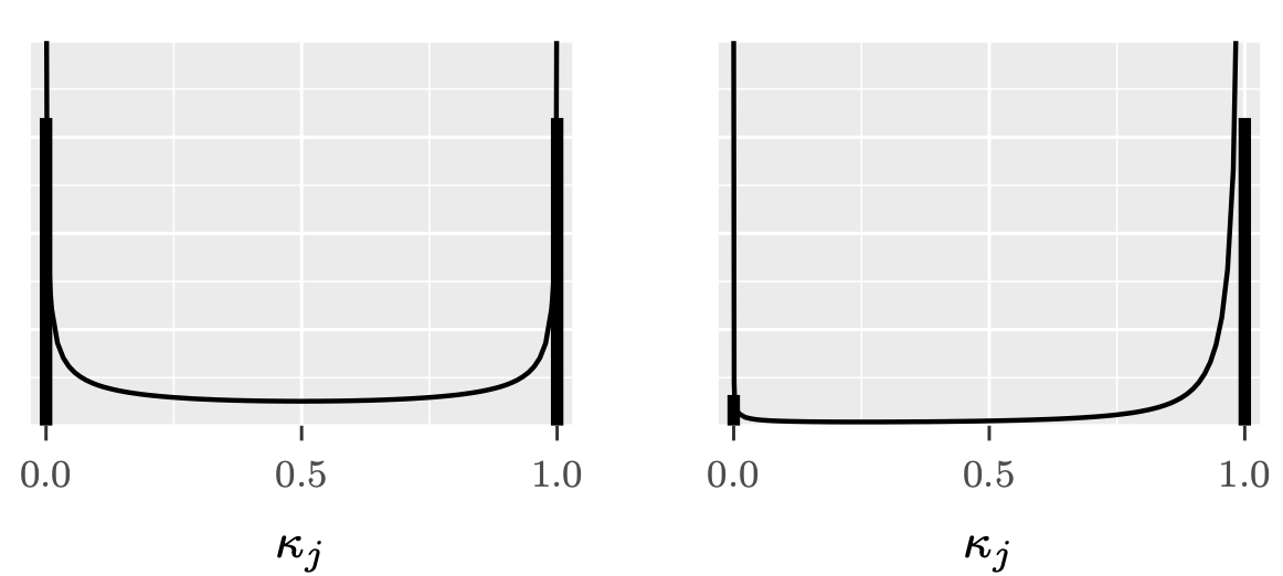
Similarity to spike-and-slab

A horseshoe prior can be considered as a continuous approximation to the spike-and-slab prior.
- The spike-and-slab places a discrete probability mass at exactly zero (the “spike”) and a separate distribution around non-zero values (the “slab”).
- The horseshoe prior smoothly approximates this behavior with a very concentrated distribution near zero.

workflow

From Piironena and Vehtari 2017

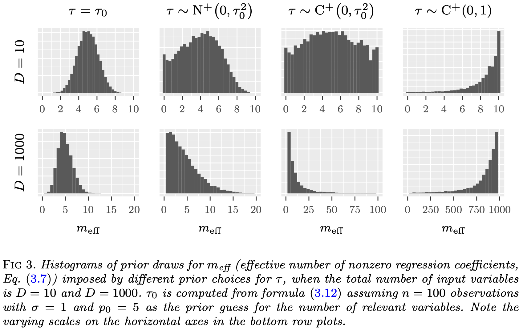
Choosing a prior for $τ$

Carvalho et al. 2009 suggest $τ \sim C^{+} (0, 1)$ .
Polson and Scott 2011 recommend $τ | σ \sim C^{+} (0, σ^{2})$ .
Another prior comes from a quantity called the effective number of nonzero coefficients,

$m_{e f f} = \sum_{j = 1}^{p} (1 - κ_{j}) .$

Global shrinkage parameter $τ$

The prior mean can be shown to be,

$E [m_{e f f} | τ, σ] = \frac{τ σ^{- 1} \sqrt{n}}{1 + τ σ^{- 1} \sqrt{n}} p .$

Setting $E [m_{e f f} | τ, σ] = p_{0}$ (prior guess for the number of non-zero coefficients) yields for $τ$ ,

$τ_{0} = \frac{p_{0}}{p - p_{0}} \frac{σ}{\sqrt{n}} .$

Global shrinkage parameter $τ$

workflow

From Piironena and Vehtari 2017

Non-Gaussian observation models

The reference value:

$τ_{0} = \frac{p_{0}}{p - p_{0}} \frac{σ}{\sqrt{n}} .$

This framework can be applied to non-Gaussian observation data models using plug-in estimates values for $σ$ .
- Gaussian approximations to the likelihood.
- For example: For logistic regression $σ = 2$ .

Coding up the model in Stan

Horseshoe model has the following form,

$\begin{aligned} β_{j} | λ_{j}, τ & \overset{i n d}{\sim} N (0, λ_{j}^{2} τ^{2}) \\ λ_{j} & \overset{i i d}{\sim} C^{+} (0, 1), \\ τ & \sim C^{+} (0, τ_{0}^{2}) . \end{aligned}$

Efficient parameter transformation, $β_{j} = τ λ_{j} z_{j}, z_{j} \overset{i i d}{\sim} N (0, 1) .$

Horseshoe in Stan

data {
  int<lower = 1> n;
  int<lower = 1> p;
  vector[n] Y;
  matrix[n, p] X;
  real<lower = 0> tau0;
}
parameters {
  real alpha;     
  real<lower = 0> sigma;
  vector[p] z;
  vector<lower = 0>[p] lambda;
  real<lower = 0> tau;
}
transformed parameters {
  vector[p] beta;
  beta = tau * lambda .* z;
}
model {
  // likelihood
  target += normal_lpdf(Y | alpha + X * beta, sigma);
  // population parameters
  target += normal_lpdf(alpha | 0, 3);
  target += normal_lpdf(sigma | 0, 3);
  // horseshoe prior
  target += std_normal_lpdf(z);
  target += cauchy_lpdf(lambda | 0, 1);
  target += cauchy_lpdf(tau | 0, tau0);
}

Prepare for next class

Work on HW 03, which was just assigned.
Complete reading to prepare for next Tuesday’s lecture
Tuesday’s lecture: Classification