BIOSTAT 725 - Spring 2025 – Scalable Gaussian Processes #1

Review of the last lecture

TBU

Motivating dataset

Recall we worked with a dataset on women aged 15-49 sampled from the 2013-14 Democratic Republic of Congo (DRC) Demographic and Health Survey. Variables are:

loc_id: location id (i.e. survey cluster).
hemoglobin: hemoglobin level (g/dL).
anemia: anemia classifications.
age: age in years.
urban: urban vs. rural.
LATNUM: latitude.
LONGNUM: longitude.

Motivating dataset

  loc_id hemoglobin     anemia age urban   LATNUM  LONGNUM
1      1       12.5 not anemic  28 rural 0.220128 21.79508
2      1       12.6 not anemic  42 rural 0.220128 21.79508
3      1       13.3 not anemic  15 rural 0.220128 21.79508
4      1       12.9 not anemic  28 rural 0.220128 21.79508
5      1       10.4       mild  32 rural 0.220128 21.79508
6      1       12.2 not anemic  42 rural 0.220128 21.79508

Modeling goals:

Learn the associations between age and urbanality and hemoglobin, accounting for unmeasured spatial confounders.
Create a predicted map of hemoglobin across the spatial surface controlling for age and urbanality, with uncertainty quantification.

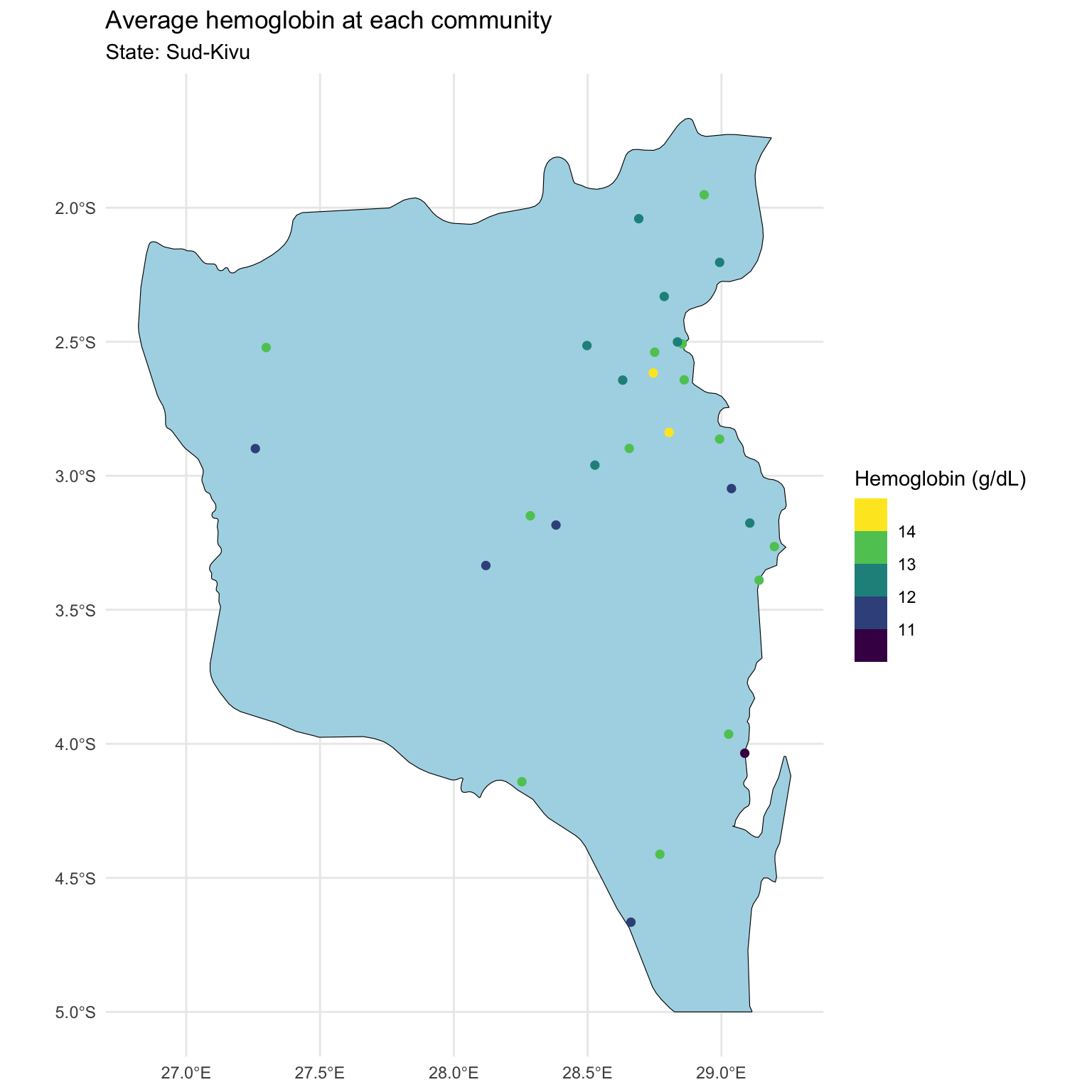
Map of Sud-Kivu state

Last time, we focused on one state with ~500 observations at ~30 locations.

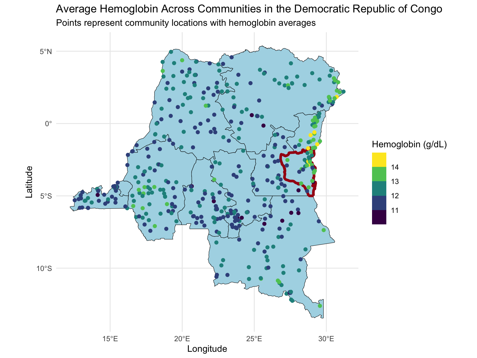
Map of the DRC

Today we will extend the analysis to the full dataset with ~8,600 observations at ~500 locations.

Modeling

$\begin{aligned} Y_{j} (u_{i}) & = α + x_{j} (u_{i}) β + θ (u_{i}) + ϵ_{j} (u_{i}), ϵ_{j} (u_{i}) \overset{i i d}{\sim} N (0, σ^{2}) \end{aligned}$

Data objects:

$i \in {1, \dots, n}$ indexes unique locations.
$j \in {1, \dots, n_{i}}$ indexes individuals at each location.
$Y_{j} (u_{i})$ denotes the observation of individual $j$ at location $u_{i}$ .
$x_{j} (u_{i}) = ({age}_{i j} / 10, {urban}_{i}) \in R^{1 \times p}$ , where $p = 2$ is the number of predictors (excluding intercept).

Modeling

$\begin{aligned} Y_{j} (u_{i}) & = α + x_{j} (u_{i}) β + θ (u_{i}) + ϵ_{j} (u_{i}), ϵ_{j} (u_{i}) \overset{i i d}{\sim} N (0, σ^{2}) \end{aligned}$

Population parameters:

$α \in R$ is the intercept.
$β \in R^{p}$ is the regression coefficients.
$σ^{2} \in R^{+}$ is the overall residual error (nugget).

Location-specific parameters:

$u_{i} = ({latitude}_{i}, {longitude}_{i}) \in R^{2}$ denotes coordinates of location $i$ .
$θ (u_{i})$ denotes the spatial intercept at location $u_{i}$ .

Location-specific notation

$Y (u_{i}) = α 1_{n_{i}} + X (u_{i}) β + θ (u_{i}) 1_{n_{i}} + ϵ (u_{i}), ϵ (u_{i}) \sim N_{n_{i}} (0, σ^{2} I)$

$Y (u_{i}) = (Y_{1} (u_{i}), \dots, Y_{n_{i}} (u_{i}))^{⊤}$ .
$X (u_{i})$ is an $n_{i} \times p$ dimensional matrix with rows $x_{j} (u_{i})$ .
$ϵ (u_{i}) = (ϵ_{i} (u_{i}), \dots, ϵ_{n_{i}} (u_{i}))^{⊤}$ .

Full data notation

$Y = α 1_{N} + X β + Z θ + ϵ, ϵ \sim N_{N} (0, σ^{2} I)$

$Y = (Y (u_{1})^{⊤}, \dots, Y (u_{n})^{⊤})^{⊤} \in R^{N}$ , with $N = \sum_{i = 1}^{n} n_{i}$ .
$X \in R^{N \times p}$ stacks $X (u_{i})$ .
$θ = (θ (u_{1}), \dots, θ (u_{n}))^{⊤} \in R^{n}$ .
$Z$ is an $N \times n$ dimensional block diagonal binary matrix. Each row contains a single 1 in column $i$ that corresponds to the location of $Y_{j} (u_{i})$ . $\begin{array}{r} Z = [\begin{array}{c} 1_{n_{1}} & 0 & \dots & 0 \\ 0 & 1_{n_{2}} & \dots & 0 \\ ⋮ & ⋮ & ⋱ & ⋮ \\ 0 & \dots & 0 & 1_{n_{n}} \end{array}] . \end{array}$

Modeling

We specify the following model: $Y = α 1_{N} + X β + Z θ + ϵ, ϵ \sim N_{N} (0, σ^{2} I)$ with priors

$θ (u) | τ, ρ \sim G P (0, C (\cdot, \cdot))$ , where $C$ is the Matérn 3/2 covariance function with magnitude $τ$ and length scale $ρ$
$α^{*} \sim N (0, 4^{2})$ . This is the intercept after centering $X$ .
$β_{j} | σ_{β} \sim N (0, σ_{β}^{2})$ , $j \in {1, \dots, p}$
$σ \sim Half-Normal (0, 2^{2})$
$τ \sim Half-Normal (0, 4^{2})$
$ρ \sim Inv-Gamma (5, 5)$
$σ_{β} \sim Half-Normal (0, 2^{2})$

Computational issues with GP

Effectively, the prior for $θ$ is $θ | τ, ρ \sim N_{n} (0, C), C \in R^{n \times n} .$ Matérn 3/2 is an isotropic covariance function, $C (u_{i}, u_{j}) = C (∥ u_{i} - u_{j} ∥)$ .

$C = [\begin{matrix} C (0) & C (∥ u_{1} - u_{2} ∥) & \dots & C (∥ u_{1} - u_{n} ∥) \\ C (∥ u_{1} - u_{2} ∥) & C (0) & \dots & C (∥ u_{2} - u_{n} ∥) \\ ⋮ & ⋮ & ⋱ & ⋮ \\ C (∥ u_{1} - u_{n} ∥) & C (∥ u_{2} - u_{n} ∥) & \dots & C (0) \end{matrix}] .$

This is not scalable because we need to invert an $n \times n$ dense covariance matrix for each MCMC iteration, which requires $O (n^{3})$ floating point operations (flops), and $O (n^{2})$ memory.

Scalable GP methods overview

The computational issues motivated exploration in scalable GP methods. Existing scalable methods broadly fall under two categories.

Sparsity methods

sparsity in $C$ , e.g., covariance tapering (@furrer2006covariance).
sparsity in $C^{- 1}$ , e.g., Vecchia approximation (@vecchia1988estimation) and nearest-neighbor GP (@datta2016hierarchical).

Low-rank methods

approximate $C$ on a low-dimensional subspace.
e.g., process convolution (@higdon2002space), inducing point method(@snelson2005sparse).

Hilbert space method for GP

@solin2020hilbert introduced a Hilbert space method for reduced-rank Gaussian process regression (HSGP).
@riutort2023practical discussed how to practically implement HSGP.
Tutorial codes are available in different probabilistic programming languages:
- stan
- NumPyro
- pyMC

Lecture plan

Today:

How does HSGP work
Why HSGP is scalable
How to use HSGP for Bayesian geospatial model fitting and posterior predictive sampling

Thursday:

Parameter tuning for HSGP
How to implement HSGP in stan

HSGP approximation

Given:

an isotropic covariance function $C$ which admits a power spectral density, e.g., the Matérn family, and
a compact domain $Θ \in R^{d}$ with smooth boundaries. For our purposes, we only consider boxes, e.g., $[- 1, 1] \times [- 1, 1]$ .

HSGP approximates the $(i, j)$ element of the corresponding $n \times n$ covariance matrix $C$ as $C_{i j} = C (∥ u_{i} - u_{j} ∥) \approx \sum_{k = 1}^{m} s_{k} ϕ_{k} (u_{i}) ϕ_{k} (u_{j}) .$

HSGP approximation

$C_{i j} = C (∥ u_{i} - u_{j} ∥) \approx \sum_{k = 1}^{m} s_{k} ϕ_{k} (u_{i}) ϕ_{k} (u_{j}) .$

$s_{k} \in R^{+}$ are positive scalars which depends on the covariance function $C$ and its parameters $τ$ and $ρ$ .
$ϕ_{k} : Θ \to R$ are basis functions which only depends on $Θ$ .
$m$ is the number of basis functions. Note: even with an infinite sum ( $m \to \infty$ ), this remains an approximation (see @solin2020hilbert).

HSGP approximation

In matrix notation,

$C \approx Φ S Φ^{⊤} .$

$Φ \in R^{n \times m}$ is a feature matrix. Only depends on $Θ$ and the observed locations.
$S \in R^{m \times m}$ is diagonal. Depends on the covariance function $C$ and parameters $τ$ and $ρ$ .

$\begin{array}{r} Φ = [\begin{array}{c} ϕ_{1} (u_{1}) & \dots & ϕ_{m} (u_{1}) \\ ⋮ & ⋱ & ⋮ \\ ϕ_{1} (u_{n}) & \dots & ϕ_{m} (u_{n}) \end{array}], S = [\begin{array}{c} s_{1} \\ ⋱ \\ s_{m} \end{array}] . \end{array}$

Why HSGP is scalable

$C \approx Φ S Φ^{⊤} .$

$Φ$ only depends on $Θ$ and the observed locations, can be pre-calculated.
No matrix inversion.
Each MCMC iteration requires $O (n m + m)$ flops, vs $O (n^{3})$ for a full GP.
Ideally $m ≪ n$ , but HSGP can be faster even for $m > n$ .

Model reparameterization

Under HSGP, approximately $θ \overset{d}{=} Φ S^{1 / 2} b, b \sim N_{m} (0, I) .$

Therefore we can reparameterize the model as

$\begin{aligned} Y & = α 1_{N} + X β + Z θ + ϵ \\ \approx α 1_{N} + X β + \underset{W}{\underset{⏟}{Z Φ S^{1 / 2}}} b + ϵ \end{aligned}$

Note the resemblance to linear regression:

$W \in R^{n \times m}$ is a known design matrix given parameters $τ$ and $ρ$ .
$b$ is an unknown parameter vector with prior $N_{m} (0, I)$ .

HSGP in `stan`

Similarly, we can use the reparameterized model in stan.

This is called the non-centered parameterization in stan documentation. It’s recommended for computational efficiency for hierarchical models.

transformed data {
  matrix[n,m] PHI;
  matrix[N,m] Z;
}
parameters {
  real alpha;
  real<lower=0> sigma;
  vector[p] beta;
  vector[m] b;
  vector<lower=0>[m] sqrt_S;
}
model {
  vector[n] theta = PHI * (sqrt_S .* b);
  target += normal_lupdf(y | alpha + X * beta + Z * theta, sigma);
  target += normal_lupdf(b | 0, 1);
  ...
}

Posterior predictive distribution

We want to make predictions for $Y^{*} = (Y (u_{n + 1}), \dots, Y (u_{n + q}))^{⊤}$ , observations at $q$ new locations. Define $θ^{*} = (θ (u_{n + 1}), \dots, θ (u_{n + q}))^{⊤}$ , $Ω = (α, β, σ, τ, ρ)$ . Recall:

$\begin{aligned} f (Y^{*} | Y) & = \int f (Y^{*}, θ^{*}, θ, Ω | Y) d θ^{*} d θ d Ω \\ = \int \underset{(1)}{\underset{⏟}{f (Y^{*} | θ^{*}, Ω)}} \underset{(2)}{\underset{⏟}{f (θ^{*} | θ, Ω)}} \underset{(3)}{\underset{⏟}{f (θ, Ω | Y)}} d θ^{*} d θ d Ω \end{aligned}$

Likelihood: $f (Y^{*} | θ^{*}, Ω)$ – remains the same as for GP
Kriging: $f (θ^{*} | θ, Ω)$ – we will focus on this next
Posterior distribution: $f (θ, Ω | Y)$ – we have just discussed

Kriging

Recall under the GP prior,

$[\begin{matrix} θ \\ θ^{*} \end{matrix}] | Ω \sim N_{n + q} ([\begin{matrix} 0_{n} \\ 0_{q} \end{matrix}], [\begin{matrix} C & C_{+} \\ C_{+}^{⊤} & C^{*} \end{matrix}]),$

where $C$ is the covariance of $θ$ , $C^{*}$ is the covariance of $θ^{*}$ , and $C_{+}$ is the cross covariance matrix between $θ$ and $θ^{*}$ .

Therefore by properties of multivariate normal, $θ^{*} ∣ (θ, Ω) \sim N_{q} (E_{θ^{*}}, V_{θ^{*}}), where$ $\begin{aligned} E_{θ^{*}} & = C_{+}^{⊤} C^{- 1} θ \\ V_{θ^{*}} & = C^{*} - C_{+}^{⊤} C^{- 1} C_{+} . \end{aligned}$

Kriging under HSGP

Under HSGP, $C^{*} \approx Φ^{*} S Φ^{* ⊤}$ , $C_{+} \approx Φ S Φ^{* ⊤}$ , where $\begin{array}{r} Φ^{*} \in R^{q \times m} = [\begin{array}{c} ϕ_{1} (u_{n + 1}) & \dots & ϕ_{m} (u_{n + 1}) \\ ⋮ & ⋱ & ⋮ \\ ϕ_{1} (u_{n + q}) & \dots & ϕ_{m} (u_{n + q}) \end{array}] \end{array}$ is the feature matrix for the new locations. Therefore approximately $\begin{array}{r} [\begin{array}{c} θ \\ θ^{*} \end{array}] \sim N_{n + q} ([\begin{array}{c} 0_{n} \\ 0_{q} \end{array}], [\begin{array}{c} Φ S Φ^{⊤} & Φ S Φ^{* ⊤} \\ Φ^{*} S Φ^{⊤} & Φ^{*} S Φ^{* ⊤} \end{array}]) . \end{array}$ Claim $θ^{*} ∣ (θ, Ω) = (Φ^{*} S Φ^{⊤}) (Φ S Φ^{⊤})^{†} θ$ , where $A^{†}$ denotes a generalized inverse of matrix $A$ such that $A A^{†} = I$ .

Kriging under HSGP

Claim $θ^{*} ∣ (θ, Ω) = (Φ^{*} S Φ^{⊤}) (Φ S Φ^{⊤})^{†} θ .$

Sketch proof below, see details in class:

By properties of multivariate normal, $θ^{*} ∣ (θ, Ω) \sim N_{q} (E_{θ^{*}}^{H S}, V_{θ^{*}}^{H S})$ , $\begin{aligned} E_{θ^{*}}^{H S} & = (Φ^{*} S Φ^{⊤}) (Φ S Φ^{⊤})^{†} θ \\ V_{θ^{*}}^{H S} & = (Φ^{*} S Φ^{* ⊤}) - (Φ^{*} S Φ^{⊤}) (Φ S Φ^{⊤})^{†} (Φ S Φ^{* ⊤}) . \end{aligned}$
Show if $Φ$ has full column rank, which is true under HSGP, then for any matrix $A$ of proper dimension, $\begin{matrix} (1) & S Φ^{⊤} (Φ S Φ^{⊤})^{†} Φ A = A \end{matrix}$ Therefore $V_{θ^{*}}^{H S} \equiv 0$ .

Kriging under HSGP

Under the reparameterized model, $θ = Φ S^{1 / 2} b$ , for $b \sim N_{m} (0, I) .$ Therefore $\begin{aligned} θ^{*} ∣ (θ, Ω) & = (Φ^{*} S Φ^{⊤}) (Φ S Φ^{⊤})^{†} θ \\ = (Φ^{*} S Φ^{⊤}) (Φ S Φ^{⊤})^{†} (Φ S^{1 / 2} b) \\ = Φ^{*} S^{1 / 2} b . (by equation (1) in the last slide) \end{aligned}$

During MCMC sampling, we can obtain posterior predictive samples for $θ^{*}$ through posterior samples of $b$ and $S$ . Let superscript $(s)$ denote the $s$ th posterior sample:

$θ^{* (s)} = Φ^{*} S^{(s) 1 / 2} b^{(s)} .$

Kriging under HSGP – alternative view

Under the reparameterized model, there is another (perhaps more intuitive) way to recognize the kriging distribution under HSGP.

We model $θ = Φ S^{1 / 2} b$ , where $b$ is treated as the unknown parameter. Therefore for kriging: $\begin{aligned} θ^{*} ∣ (θ, Ω) & = Φ^{*} S^{1 / 2} b ∣ (b, Ω) \\ = Φ^{*} S^{1 / 2} b . \end{aligned}$

HSGP kriging in `stan`

Kriging under HSGP can be easily implemented in stan.

transformed data {
  matrix[q,m] PHI_new;
}
parameters {
  vector[m] b;
  vector<lower=0>[m] sqrt_S;
}
generated quantities {
  vector[q] theta_new = PHI_new * (sqrt_S .* b);
}

Recap

HSGP is a low rank approximation method for GP.

$\begin{array}{r} C_{i j} \approx \sum_{k = 1}^{m} s_{k} ϕ_{k} (u_{i}) ϕ_{k} (u_{j}), C \approx Φ S Φ^{⊤}, \end{array}$

for covariance function $C$ which admits a power spectral density.
on a box $Θ \subset R^{d}$ .
with $m$ number of basis functions.

We have talked about:

why HSGP is scalable.
how to do posterior sampling and posterior predictive sampling in stan.

HSGP parameters

@solin2020hilbert showed that HSGP approximation can be made arbitrarily accurate as $Θ$ and $m$ increase.

But how to choose:

size of the box $Θ$ .
number of basis functions $m$ .

HSGP approximation box

Due to the design of HSGP, the approximation is less accurate near the boundaries of $Θ$ .

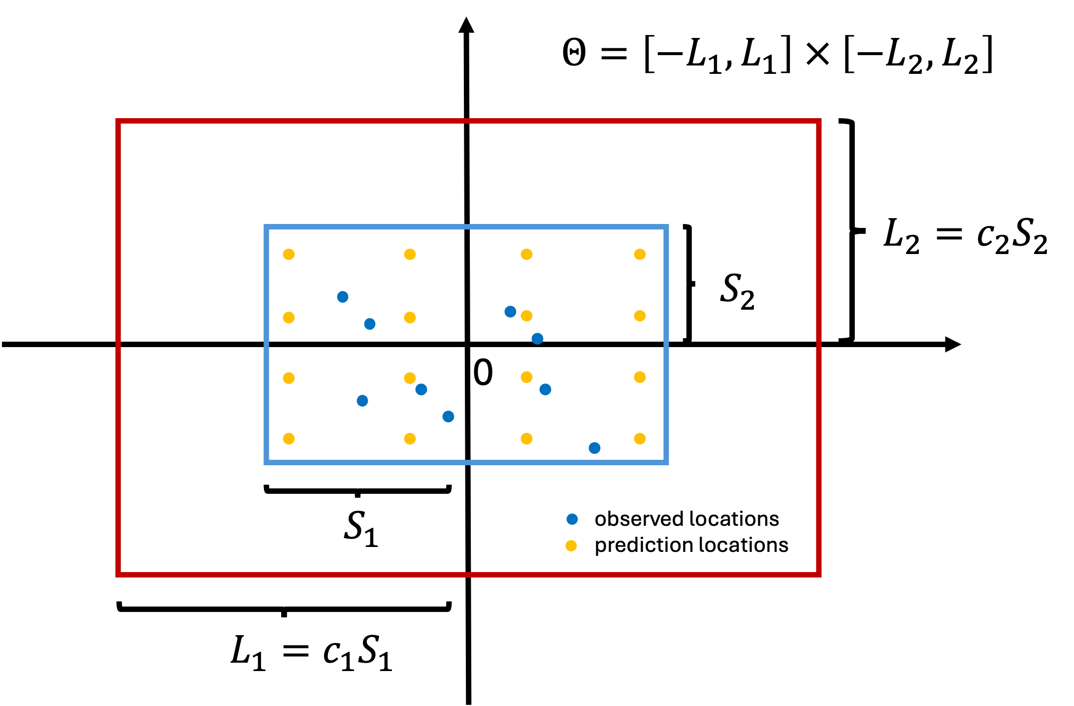
Suppose all the coordinates are centered. Let $S_{l} = max_{i} | u_{i l} |, l = 1, \dots, d, i = 1, \dots, (n + q)$ such that $Θ_{S} = \prod_{l = 1}^{d} [- S_{l}, S_{l}]$ is the smallest box which contains all observed and prediction locations. We should at least ensure $Θ \supset Θ_{S}$ .
We want the box to be large enough to ensure good boundary accuracy. Let $c_{l} \geq 1$ be boundary factors, we consider $Θ = \prod_{l = 1}^{d} [- L_{l}, L_{l}], L_{l} = c_{l} S_{l} .$

HSGP approximation box

How much the approximation accuracy deteriorates towards the boundaries depends on smoothness of the true surface.

E.g., the larger the length scale $ρ$ , the smoother the surface, a smaller box can be used for the same level of boundary accuracy.

HSGP approximation box

The larger the box,

the more basis functions we need for the same level of overall accuracy,
hence higher run time.

HSGP basis functions

The total number of basis functions $m = \prod_{l = 1}^{d} m_{l}$ , i.e., we need to decide on $m_{l}$ ’s, the number of basis functions for each dimension.

The higher the $m$ , the better the overall approximation accuracy, the higher the runtime.
$m$ scales exponentially in $d$ , hence the HSGP computation complexity $O (m n + m)$ also scales exponentially in $d$ . Therefore HSGP is only recommended for $d \leq 3$ , at most $4$ .

Relationship between $c$ and $m$

@riutort2023practical used simulations with a squared exponential covariance function to investigate the relationship between $c$ and $m$ .

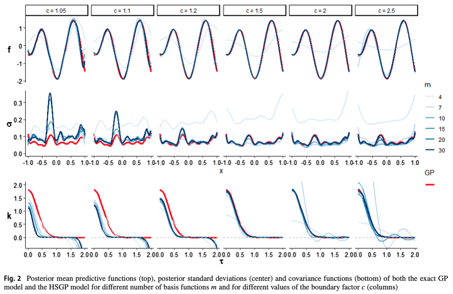
Notice that $c$ needs to be above a certain minimum value to achieve a reasonable boundary accuracy.

Relationship between $c$ , $m$ and $ρ$

To summarize:

The boundary factor $c$ needs to be above a minimum value, otherwise HSGP approximation is poor no matter how large $m$ is.
As $ρ$ increases, the surface is less smooth,

$c$ needs to increase to retain boundary accuracy.
$m$ needs to increase to retain overall accuracy.

As $c$ increases, $m$ needs to increase to retain overall accuracy.
As $m$ increases, run time increases. Hence we want to minimize $m$ and $c$ while maintaining certain accuracy level.

And, we do not know $ρ$ . So how to choose $c$ and $m$ ?

Prepare for next class

Work on HW 05 which is due Apr 8
Complete reading to prepare for Thursday’s lecture
Thursday’s lecture:

Parameter tuning for HSGP
How to implement HSGP in stan