Scalable Gaussian Processes #1

Christine Shen

Apr 01, 2025

Review of previous lectures

Two weeks ago, we learned about:

1. Gaussian processes, and

2. How to use Gaussian processes for

   • longitudinal data
   • geospatial data

Motivating dataset

Recall we worked with a dataset on women aged 15-49 sampled from the 2013-14 Democratic Republic of Congo (DRC) Demographic and Health Survey. Variables are:

• loc_id: location id (i.e. survey cluster).

• hemoglobin: hemoglobin level (g/dL).

• anemia: anemia classifications.

• age: age in years.

• urban: urban vs. rural.

• LATNUM: latitude.

• LONGNUM: longitude.

Motivating dataset

  loc_id hemoglobin     anemia age urban   LATNUM  LONGNUM
1      1       12.5 not anemic  28 rural 0.220128 21.79508
2      1       12.6 not anemic  42 rural 0.220128 21.79508
3      1       13.3 not anemic  15 rural 0.220128 21.79508
4      1       12.9 not anemic  28 rural 0.220128 21.79508
5      1       10.4       mild  32 rural 0.220128 21.79508
6      1       12.2 not anemic  42 rural 0.220128 21.79508

Modeling goals:

• Learn the associations between age and urbanicity and hemoglobin, accounting for unmeasured spatial confounders.

• Create a predicted map of hemoglobin across the spatial surface controlling for age and urbanicity, with uncertainty quantification.

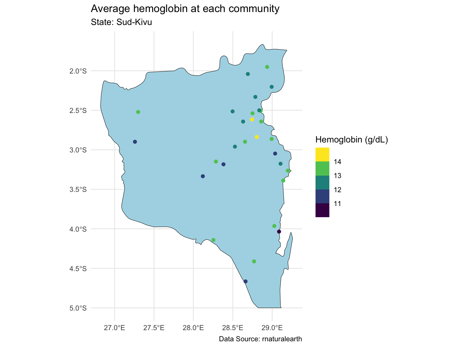
Map of the Sud-Kivu state

Last time, we focused on one state with ~500 observations at ~30 locations.

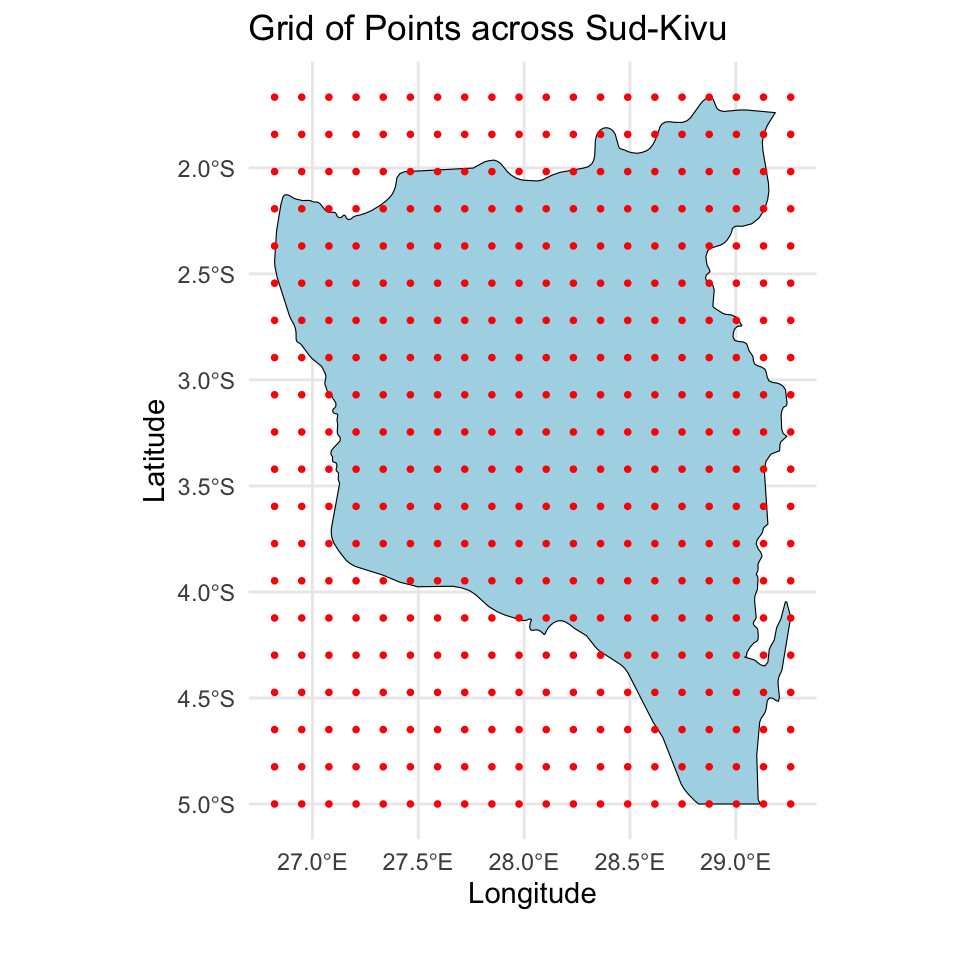
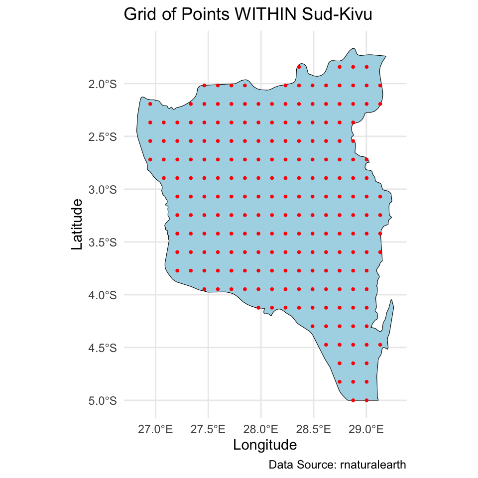
Prediction for the Sud-Kivu state

And we created a \(20 \times 20\) grid for prediction of the spatial intercept surface over the Sud-Kivu state.

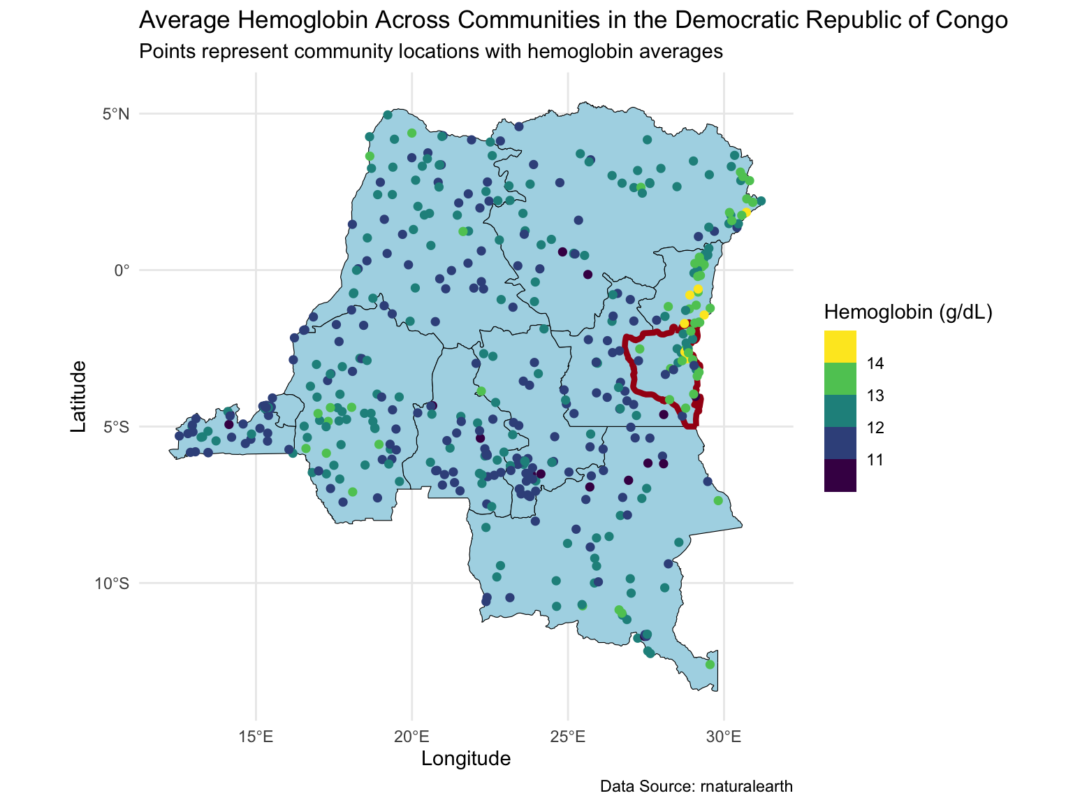
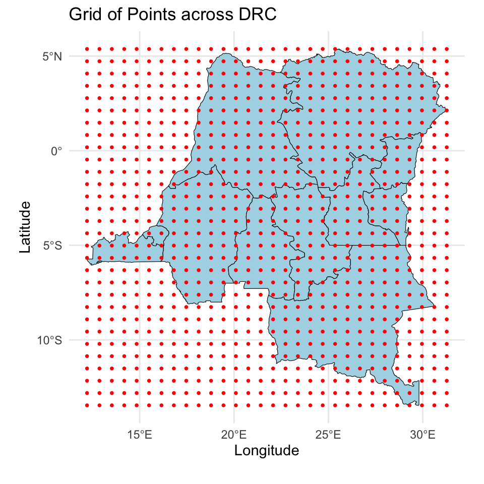
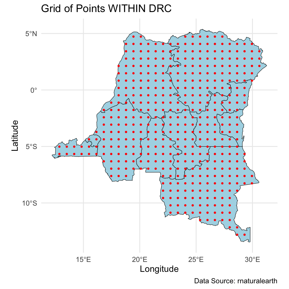
Map of the DRC

Today we will extend the analysis to the full dataset with ~8,600 observations at ~500 locations.

Prediction for the DRC

And we will make predictions on a \(30 \times 30\) grid over the DRC.

Modeling

\[\begin{align*} Y_j(\mathbf{u}_i) &= \alpha + \mathbf{x}_j(\mathbf{u}_i) \boldsymbol{\beta} + \theta(\mathbf{u}_i) + \epsilon_j(\mathbf{u}_i), \quad \epsilon_j(\mathbf{u}_i) \stackrel{iid}{\sim} N(0,\sigma^2) \end{align*}\]

Data objects:

• \(i \in \{1,\dots,n\}\) indexes unique locations.

• \(j \in \{1,\dots,n_i\}\) indexes individuals at each location.

• \(Y_j(\mathbf{u}_i)\) denotes the hemoglobin level of individual \(j\) at location \(\mathbf{u}_i\).

• \(\mathbf{x}_j(\mathbf{u}_i) = (\text{age}_{ij}/10,\text{urban}_i) \in \mathbb{R}^{1 \times p}\), where \(p=2\) is the number of predictors (excluding intercept).

Modeling

\[\begin{align*} Y_j(\mathbf{u}_i) &= \alpha + \mathbf{x}_j(\mathbf{u}_i) \boldsymbol{\beta} + \theta(\mathbf{u}_i) + \epsilon_j(\mathbf{u}_i), \quad \epsilon_j(\mathbf{u}_i) \stackrel{iid}{\sim} N(0,\sigma^2) \end{align*}\]

Population parameters:

• \(\alpha \in \mathbb{R}\) is the intercept.

• \(\boldsymbol{\beta} \in \mathbb{R}^p\) is the regression coefficients.

• \(\sigma^2 \in \mathbb{R}^+\) is the overall residual error (nugget).

Location-specific parameters:

• \(\mathbf{u}_i = (\text{longitude}_i,\text{latitude}_i) \in \mathbb{R}^2\) denotes coordinates of location \(i\).

• \(\theta(\mathbf{u}_i)\) denotes the spatial intercept at location \(\mathbf{u}_i\).

Location-specific notation

\[\mathbf{Y}(\mathbf{u}_i) = \alpha \mathbf{1}_{n_i} + \mathbf{X}(\mathbf{u}_i) \boldsymbol{\beta} + \theta(\mathbf{u}_i)\mathbf{1}_{n_i} + \boldsymbol{\epsilon}(\mathbf{u}_i), \quad \boldsymbol{\epsilon}(\mathbf{u}_i) \sim N_{n_i}(\mathbf{0},\sigma^2\mathbf{I})\]

• \(\mathbf{Y}(\mathbf{u}_i) = (Y_1(\mathbf{u}_i),\ldots,Y_{n_i}(\mathbf{u}_i))^\top\).

• \(\mathbf{X}(\mathbf{u}_i)\) is an \(n_i \times p\) dimensional matrix with rows \(\mathbf{x}_j(\mathbf{u}_i)\).

• \(\boldsymbol{\epsilon}(\mathbf{u}_i) = (\epsilon_i(\mathbf{u}_i),\ldots,\epsilon_{n_i}(\mathbf{u}_i))^\top\).

Full data notation

\[\mathbf{Y} = \alpha \mathbf{1}_{N} + \mathbf{X} \boldsymbol{\beta} + \mathbf{Z}\boldsymbol{\theta} + \boldsymbol{\epsilon}, \quad \boldsymbol{\epsilon} \sim N_N(\mathbf{0},\sigma^2\mathbf{I})\]

• \(\mathbf{Y} = (\mathbf{Y}(\mathbf{u}_1)^\top,\ldots,\mathbf{Y}(\mathbf{u}_{n})^\top)^\top \in \mathbb{R}^N\), with \(N = \sum_{i=1}^n n_i\).

• \(\mathbf{X} \in \mathbb{R}^{N \times p}\) stacks \(\mathbf{X}(\mathbf{u}_i)\).

• \(\boldsymbol{\theta} = (\theta(\mathbf{u}_1),\ldots,\theta(\mathbf{u}_n))^\top \in \mathbb{R}^n\).

• \(\mathbf{Z}\) is an \(N \times n\) dimensional block diagonal binary matrix. Each row contains a single 1 in column \(i\) that corresponds to the location of \(Y_j(\mathbf{u}_i)\). \[ \begin{align} \mathbf{Z} = \begin{bmatrix} \mathbf{1}_{n_1} & \mathbf{0} & \dots & \mathbf{0} \\ \mathbf{0} & \mathbf{1}_{n_2} & \dots & \mathbf{0} \\ \vdots & \vdots & \ddots & \vdots \\ \mathbf{0} & \dots & \mathbf{0} & \mathbf{1}_{n_n} \end{bmatrix}. \end{align} \]

Modeling

We specify the following model: \[\mathbf{Y} = \alpha \mathbf{1}_{N} + \mathbf{X} \boldsymbol{\beta} + \mathbf{Z}\boldsymbol{\theta} + \boldsymbol{\epsilon}, \quad \boldsymbol{\epsilon} \sim N_N(\mathbf{0},\sigma^2\mathbf{I})\] with priors

• \(\boldsymbol{\theta}(\mathbf{u}) | \tau,\rho \sim GP(\mathbf{0},C(\cdot,\cdot))\), where \(C\) is the Matérn 3/2 covariance function with magnitude \(\tau\) and length scale \(\rho\).
• \(\alpha^* \sim N(0,4^2)\). This is the intercept after centering \(\mathbf{X}\).
• \(\beta_j | \sigma_{\beta} \sim N(0,\sigma_{\beta}^2)\), \(j \in \{1,\dots,p\}\)
• \(\sigma \sim \text{Half-Normal}(0, 2^2)\)
• \(\tau \sim \text{Half-Normal}(0, 4^2)\)
• \(\rho \sim \text{Inv-Gamma}(5, 5)\)
• \(\sigma_{\beta} \sim \text{Half-Normal}(0, 2^2)\)

Computational issues with GP

Effectively, the prior for \(\boldsymbol{\theta}\) is \[\boldsymbol{\theta} | \tau,\rho \sim N_n(\mathbf{0},\mathbf{C}), \quad \mathbf{C} \in \mathbb{R}^{n \times n}.\] Matérn 3/2 is an isotropic covariance function, \(C(\mathbf{u}_i, \mathbf{u}_j) = C(\|\mathbf{u}_i-\mathbf{u}_j\|)\).

\[\mathbf{C} = \begin{bmatrix} C(\mathbf{0}) & C(\|\mathbf{u}_1 - \mathbf{u}_2\|) & \cdots & C(\|\mathbf{u}_1 - \mathbf{u}_n\|)\\ C(\|\mathbf{u}_1 - \mathbf{u}_2\|) & C(\mathbf{0}) & \cdots & C(\|\mathbf{u}_2 - \mathbf{u}_n\|)\\ \vdots & \vdots & \ddots & \vdots\\ C(\|\mathbf{u}_{1} - \mathbf{u}_n\|) & C(\|\mathbf{u}_2 - \mathbf{u}_n\|) & \cdots & C(\mathbf{0})\\ \end{bmatrix}.\]

This is not scalable because we need to invert an \(n \times n\) dense covariance matrix for each MCMC iteration, which requires \(\mathcal{O}(n^3)\) floating point operations (flops), and \(\mathcal{O}(n^2)\) memory.

Scalable GP methods overview

The computational issues motivated exploration in scalable GP methods. Existing scalable methods broadly fall under two categories.

1. Sparsity methods

   • sparsity in \(\mathbf{C}\), e.g., covariance tapering (Furrer, Genton, and Nychka (2006)).
   • sparsity in \(\mathbf{C}^{-1}\), e.g., Vecchia approximation (Vecchia (1988)) and nearest-neighbor GP (Datta et al. (2016)).

2. Low-rank methods

   • approximate \(\mathbf{C}\) on a low-dimensional subspace.
   • e.g., process convolution (Higdon (2002)), inducing point method(Snelson and Ghahramani (2005)).

Hilbert space method for GP

• Solin and Särkkä (2020) introduced a Hilbert space method for reduced-rank Gaussian process regression (HSGP).

• Riutort-Mayol et al. (2023) discussed how to practically implement HSGP.

• Tutorial codes are available in different probabilistic programming languages:

  • stan
  • NumPyro
  • pyMC

Lecture plan

Today:

• How does HSGP work
• Why HSGP is scalable
• How to use HSGP for Bayesian geospatial model fitting and posterior predictive sampling

Thursday:

• Parameter tuning for HSGP
• How to implement HSGP in stan

HSGP approximation

Given:

• an isotropic covariance function \(C\) which admits a power spectral density, e.g., the Matérn family, and
• a compact domain \(\boldsymbol{\Theta} \in \mathbb{R}^d\) with smooth boundaries. For our purposes, we only consider boxes, e.g., \([-1,1] \times [-1,1]\).

HSGP approximates the \((i,j)\) element of the corresponding \(n \times n\) covariance matrix \(\mathbf{C}\) as \[\mathbf{C}_{ij}=C(\|\mathbf{u}_i - \mathbf{u}_j\|) \approx \sum_{k=1}^m s_k\phi_k(\mathbf{u}_i)\phi_k(\mathbf{u}_j).\]

HSGP approximation

\[\mathbf{C}_{ij}=C(\|\mathbf{u}_i - \mathbf{u}_j\|) \approx \sum_{k=1}^m s_k\phi_k(\mathbf{u}_i)\phi_k(\mathbf{u}_j).\]

• \(s_k \in \mathbb{R}^+\) are positive scalars which depends on the covariance function \(C\) and its parameters \(\tau\) and \(\rho\).
• \(\phi_k: \boldsymbol{\Theta} \to \mathbb{R}\) are basis functions which only depends on \(\boldsymbol{\Theta}\).
• \(m\) is the number of basis functions. Note: even with an infinite sum (i.e., \(m \to \infty\)), this remains an approximation (see Solin and Särkkä (2020)).

HSGP approximation

In matrix notation,

\[\mathbf{C} \approx \boldsymbol{\Phi} \mathbf{S} \boldsymbol{\Phi}^\top.\]

• \(\boldsymbol{\Phi} \in \mathbb{R}^{n \times m}\) is a feature matrix. Only depends on \(\boldsymbol{\Theta}\) and the observed locations.
• \(\mathbf{S} \in \mathbb{R}^{m \times m}\) is diagonal. Depends on the covariance function \(C\) and parameters \(\tau\) and \(\rho\).

\[ \begin{align} \boldsymbol{\Phi} = \begin{bmatrix} \phi_1(\mathbf{u}_1) & \dots & \phi_m(\mathbf{u}_1) \\ \vdots & \ddots & \vdots \\ \phi_1(\mathbf{u}_n) & \dots & \phi_m(\mathbf{u}_n) \end{bmatrix}, \quad \mathbf{S} = \begin{bmatrix} s_1 & & \\ & \ddots & \\ & & s_m \end{bmatrix}. \end{align} \]

Why HSGP is scalable

\[\mathbf{C} \approx \boldsymbol{\Phi} \mathbf{S} \boldsymbol{\Phi}^\top.\]

• \(\boldsymbol{\Phi}\) only depends on \(\boldsymbol{\Theta}\) and the observed locations, can be pre-calculated.
• No matrix inversion.
• Each MCMC iteration requires \(\mathcal{O}(nm + m)\) flops, vs \(\mathcal{O}(n^3)\) for a full GP.
• Ideally \(m \ll n\), but HSGP can be faster even for \(m>n\).

Model reparameterization

Under HSGP, approximately \[\boldsymbol{\theta} \overset{d}{=} \boldsymbol{\Phi} \mathbf{S}^{1/2}\mathbf{b}, \quad \mathbf{b} \sim N_m(0,\mathbf{I}).\]

Therefore we can reparameterize the model as

\[ \begin{align} \mathbf{Y} &= \alpha \mathbf{1}_{N} + X\boldsymbol{\beta} + \mathbf{Z}\boldsymbol{\theta} + \boldsymbol{\epsilon} \\ &\approx \alpha \mathbf{1}_{N} + X\boldsymbol{\beta} + \underbrace{\mathbf{Z}\boldsymbol{\Phi} \mathbf{S}^{1/2}}_{\mathbf{W}}\mathbf{b} + \boldsymbol{\epsilon} \end{align} \]

Note the resemblance to linear regression:

• \(\mathbf{W} \in \mathbb{R}^{n \times m}\) is a known design matrix given parameters \(\tau\) and \(\rho\).
• \(\mathbf{b}\) is an unknown parameter vector with prior \(N_m(0,\mathbf{I})\).

HSGP in stan

Similarly, we can use the reparameterized model in stan.

This is called the non-centered parameterization in stan documentation. It’s recommended for computational efficiency for hierarchical models.

transformed data {
  matrix[n,m] PHI;
  matrix[N,m] Z;
  matrix[N,p] X_centered;
}
parameters {
  real alpha_star;
  real<lower=0> sigma;
  vector[p] beta;
  vector[m] b;
  vector<lower=0>[m] sqrt_S;
  ...
}
model {
  vector[n] theta = PHI * (sqrt_S .* b);
  target += normal_lupdf(y | alpha_star + X_centered * beta + Z * theta, sigma);
  target += normal_lupdf(b | 0, 1);
  ...
}

Posterior predictive distribution

We want to make predictions for \(\mathbf{Y}^* = (Y(\mathbf{u}_{n+1}),\ldots, Y(\mathbf{u}_{n+q}))^\top\), observations at \(q\) new locations. Define \(\boldsymbol{\theta}^* = (\theta(\mathbf{u}_{n+1}),\ldots,\theta(\mathbf{u}_{n+q}))^\top\), \(\boldsymbol{\Omega} = (\alpha,\boldsymbol{\beta},\sigma,\tau,\rho)\). Recall:

\[\begin{align*} f(\mathbf{Y}^* | \mathbf{Y}) &= \int f(\mathbf{Y}^*, \boldsymbol{\theta}^*, \boldsymbol{\theta}, \boldsymbol{\Omega} | \mathbf{Y}) d\boldsymbol{\theta}^* d\boldsymbol{\theta} d\boldsymbol{\Omega}\\ &= \int \underbrace{f(\mathbf{Y}^* | \boldsymbol{\theta}^*, \boldsymbol{\Omega})}_{(1)} \underbrace{f(\boldsymbol{\theta}^* | \boldsymbol{\theta}, \boldsymbol{\Omega})}_{(2)} \underbrace{f(\boldsymbol{\theta},\boldsymbol{\Omega} | \mathbf{Y})}_{(3)} d\boldsymbol{\theta}^* d\boldsymbol{\theta} d\boldsymbol{\Omega}\\ \end{align*}\]

1. Likelihood: \(f(\mathbf{Y}^* | \boldsymbol{\theta}^*, \boldsymbol{\Omega})\) – remains the same as for GP

2. Kriging: \(f(\boldsymbol{\theta}^* | \boldsymbol{\theta}, \boldsymbol{\Omega})\) – we will focus on this next

3. Posterior distribution: \(f(\boldsymbol{\theta},\boldsymbol{\Omega} | \mathbf{Y})\) – we have just discussed

Kriging

Recall under the GP prior,

\[\begin{bmatrix} \boldsymbol{\theta}\\ \boldsymbol{\theta}^* \end{bmatrix} \Bigg| \boldsymbol{\Omega} \sim N_{n+q}\left(\begin{bmatrix} \mathbf{0}_n \\ \mathbf{0}_q \end{bmatrix}, \begin{bmatrix} \mathbf{C} & \mathbf{C}_{+}\\ \mathbf{C}_{+}^\top & \mathbf{C}^* \end{bmatrix}\right),\]

where \(\mathbf{C}\) is the covariance of \(\boldsymbol{\theta}\), \(\mathbf{C}^*\) is the covariance of \(\boldsymbol{\theta}^*\), and \(\mathbf{C}_{+}\) is the cross covariance matrix between \(\boldsymbol{\theta}\) and \(\boldsymbol{\theta}^*\).

Therefore by properties of multivariate normal, \[\boldsymbol{\theta}^* \mid (\boldsymbol{\theta}, \boldsymbol{\Omega}) \sim N_q(\mathbb{E}_{\boldsymbol{\theta}^*},\mathbb{V}_{\boldsymbol{\theta}^*}), \quad \text{where}\] \[ \begin{align} \mathbb{E}_{\boldsymbol{\theta}^*} &= \mathbf{C}_+^\top \mathbf{C}^{-1} \boldsymbol{\theta}\\ \mathbb{V}_{\boldsymbol{\theta}^*} &= \mathbf{C}^* - \mathbf{C}_+^\top \mathbf{C}^{-1} \mathbf{C}_+. \end{align} \]

Kriging under HSGP

Under HSGP, \(\mathbf{C}^* \approx \boldsymbol{\Phi}^* \mathbf{S}\boldsymbol{\Phi}^{*\top}\), \(\mathbf{C}_+ \approx \boldsymbol{\Phi} \mathbf{S}\boldsymbol{\Phi}^{*\top}\), where \[ \begin{align} \boldsymbol{\Phi}^* \in \mathbb{R}^{q \times m} = \begin{bmatrix} \phi_1(\mathbf{u}_{n+1}) & \dots & \phi_m(\mathbf{u}_{n+1}) \\ \vdots & \ddots & \vdots \\ \phi_1(\mathbf{u}_{n+q}) & \dots & \phi_m(\mathbf{u}_{n+q}) \end{bmatrix} \end{align} \] is the feature matrix for the new locations. Therefore approximately \[ \begin{align} \begin{bmatrix} \boldsymbol{\theta} \\ \boldsymbol{\theta}^* \end{bmatrix} \Bigg| \boldsymbol{\Omega} \sim N_{n +q} \left(\begin{bmatrix} \mathbf{0}_n \\ \mathbf{0}_q \end{bmatrix}, \begin{bmatrix} \boldsymbol{\Phi}\mathbf{S}\boldsymbol{\Phi}^\top & \boldsymbol{\Phi}\mathbf{S} \boldsymbol{\Phi}^{*\top} \\ \boldsymbol{\Phi}^*\mathbf{S}\boldsymbol{\Phi}^\top & \boldsymbol{\Phi}^*\mathbf{S}\boldsymbol{\Phi}^{*\top} \end{bmatrix} \right). \end{align} \]

Kriging under HSGP

Again by properties of multivariate normal, \[\boldsymbol{\theta}^* \mid (\boldsymbol{\theta}, \boldsymbol{\Omega}) \overset{?}{\sim} N_q(\mathbb{E}_{\boldsymbol{\theta}^*}^{HS},\mathbb{V}_{\boldsymbol{\theta}^*}^{HS}),\]

\[ \begin{align} \mathbb{E}_{\boldsymbol{\theta}^*}^{HS} &= (\boldsymbol{\Phi}^*\mathbf{S}\boldsymbol{\Phi}^\top) (\boldsymbol{\Phi}\mathbf{S}\boldsymbol{\Phi}^\top)^{-1} \boldsymbol{\theta}\\ \mathbb{V}_{\boldsymbol{\theta}^*}^{HS} &= (\boldsymbol{\Phi}^*\mathbf{S}\boldsymbol{\Phi}^{*\top}) - (\boldsymbol{\Phi}^*\mathbf{S}\boldsymbol{\Phi}^\top) (\boldsymbol{\Phi}\mathbf{S}\boldsymbol{\Phi}^\top)^{-1}(\boldsymbol{\Phi}\mathbf{S} \boldsymbol{\Phi}^{*\top}). \end{align} \]

• If \(m \ge n\), \((\boldsymbol{\Phi}\mathbf{S}\boldsymbol{\Phi}^\top)\) is invertible, this is the kriging distribution under HSGP.
• But what if \(m < n\)?

Kriging under HSGP

If \(m \le n\), claim \(\boldsymbol{\theta}^* \mid (\boldsymbol{\theta}, \boldsymbol{\Omega}) = (\boldsymbol{\Phi}^*\mathbf{S}\boldsymbol{\Phi}^\top) (\boldsymbol{\Phi}\mathbf{S}\boldsymbol{\Phi}^\top)^{\dagger} \boldsymbol{\theta},\) where \(\mathbf{A}^\dagger\) denotes a generalized inverse of matrix \(\mathbf{A}\) such that \(\mathbf{A}\mathbf{A}^{\dagger}\mathbf{A} = \mathbf{A}\). Sketch proof below, see details in class.

1. By properties of multivariate normal, \(\boldsymbol{\theta}^* \mid (\boldsymbol{\theta}, \boldsymbol{\Omega}) \sim N_q(\mathbb{E}_{\boldsymbol{\theta}^*}^{HS},\mathbb{V}_{\boldsymbol{\theta}^*}^{HS})\), \[ \begin{align} \mathbb{E}_{\boldsymbol{\theta}^*}^{HS} &= (\boldsymbol{\Phi}^*\mathbf{S}\boldsymbol{\Phi}^\top) (\boldsymbol{\Phi}\mathbf{S}\boldsymbol{\Phi}^\top)^{\dagger} \boldsymbol{\theta}\\ \mathbb{V}_{\boldsymbol{\theta}^*}^{HS} &= (\boldsymbol{\Phi}^*\mathbf{S}\boldsymbol{\Phi}^{*\top}) - (\boldsymbol{\Phi}^*\mathbf{S}\boldsymbol{\Phi}^\top) (\boldsymbol{\Phi}\mathbf{S}\boldsymbol{\Phi}^\top)^{\dagger \top}(\boldsymbol{\Phi}\mathbf{S} \boldsymbol{\Phi}^{*\top}). \end{align} \]

2. Show if \(\boldsymbol{\Phi}\) has full column rank, which is true under HSGP, then \[ \begin{align} \mathbf{S} \boldsymbol{\Phi}^\top(\boldsymbol{\Phi}\mathbf{S}\boldsymbol{\Phi}^\top)^{\dagger \top}\boldsymbol{\Phi}\mathbf{S} = \mathbf{S} \tag{1} \\ \mathbf{S} \boldsymbol{\Phi}^\top(\boldsymbol{\Phi}\mathbf{S}\boldsymbol{\Phi}^\top)^{\dagger}\boldsymbol{\Phi}\mathbf{S} = \mathbf{S} \tag{2}. \end{align} \] Equation (1) is sufficient to show \(\mathbb{V}_{\boldsymbol{\theta}^*}^{HS} \equiv \mathbf{0}\).

Kriging under HSGP

Under the reparameterized model, \(\boldsymbol{\theta} = \boldsymbol{\Phi} \mathbf{S}^{1/2}\mathbf{b}\), for \(\mathbf{b} \sim N_m(0,\mathbf{I}).\) Therefore \[ \begin{align} \boldsymbol{\theta}^* \mid (\boldsymbol{\theta},\boldsymbol{\Omega}) &= (\boldsymbol{\Phi}^*\mathbf{S}\boldsymbol{\Phi}^\top) (\boldsymbol{\Phi}\mathbf{S}\boldsymbol{\Phi}^\top)^{\dagger} \boldsymbol{\theta} \\ &= (\boldsymbol{\Phi}^*\mathbf{S}\boldsymbol{\Phi}^\top) (\boldsymbol{\Phi}\mathbf{S}\boldsymbol{\Phi}^\top)^{\dagger}(\boldsymbol{\Phi} \mathbf{S}^{1/2}\mathbf{b}) \\ &= \boldsymbol{\Phi}^*\mathbf{S}^{1/2}\mathbf{b}. \quad (\text{by equation (2) in the last slide}) \end{align} \]

During MCMC sampling, we can obtain posterior predictive samples for \(\boldsymbol{\theta}^*\) through posterior samples of \(\mathbf{b}\) and \(\mathbf{S}\). Let superscript \((s)\) denote the \(s\)th posterior sample:

\[\boldsymbol{\theta}^{*(s)} = \boldsymbol{\Phi}^* \mathbf{S}^{(s) 1/2} \mathbf{b}^{(s)}.\]

Kriging under HSGP – alternative view

Under the reparameterized model, there is another (perhaps more intuitive) way to recognize the kriging distribution under HSGP when \(m \le n\).

We model \(\boldsymbol{\theta} = \boldsymbol{\Phi} \mathbf{S}^{1/2}\mathbf{b}\), where \(\mathbf{b}\) is treated as the unknown parameter. Therefore for kriging: \[ \begin{align} \boldsymbol{\theta}^* \mid (\boldsymbol{\theta},\boldsymbol{\Omega}) &= \boldsymbol{\Phi}^*\mathbf{S}^{1/2}\mathbf{b} \mid (\mathbf{b},\mathbf{S},\boldsymbol{\Omega}) \\ &=\boldsymbol{\Phi}^*\mathbf{S}^{1/2}\mathbf{b}. \end{align} \]

HSGP kriging in stan

If \(m \le n\), kriging under HSGP can be easily implemented in stan.

transformed data {
  matrix[q,m] PHI_new;
  ...
}
parameters {
  vector[m] b;
  vector<lower=0>[m] sqrt_S;
  ...
}
model {
  ...
}
generated quantities {
  vector[q] theta_new = PHI_new * (sqrt_S .* b);
}

If \(m>n\), we need to invert an \(n \times n\) matrix \((\boldsymbol{\Phi}\mathbf{S}\boldsymbol{\Phi}^\top)\) for kriging, which could be computationally prohibitive.

Recap

HSGP is a low rank approximation method for GP.

\[ \begin{align} \mathbf{C}_{ij} \approx \sum_{k=1}^m s_k\phi_k(\mathbf{u}_i)\phi_k(\mathbf{u}_j), \quad \mathbf{C} \approx \boldsymbol{\Phi} \mathbf{S} \boldsymbol{\Phi}^\top, \end{align} \]

• for covariance function \(C\) which admits a power spectral density.
• on a box \(\boldsymbol{\Theta} \subset \mathbb{R}^d\).
• with \(m\) number of basis functions.

We have talked about:

• why HSGP is scalable.
• how to do posterior sampling and posterior predictive sampling in stan.

HSGP parameters

Solin and Särkkä (2020) showed that HSGP approximation can be made arbitrarily accurate as \(\boldsymbol{\Theta}\) and \(m\) increase.

But how to choose:

• size of the box \(\boldsymbol{\Theta}\).
• number of basis functions \(m\).

Our goal:

Minimize the run time while maintaining reasonable approximation accuracy.

Note: we treat estimation of the GP magnitude parameter \(\tau\) as a separate problem, and only consider approximation accuracy of HSGP in terms of the correlation function.

Prepare for next class

1. Work on HW 05 which is due Apr 8

2. Complete reading to prepare for Thursday’s lecture

3. Thursday’s lecture:

   • Parameter tuning for HSGP
   • How to implement HSGP in stan

References

Datta, Abhirup, Sudipto Banerjee, Andrew O Finley, and Alan E Gelfand. 2016. “Hierarchical Nearest-Neighbor Gaussian Process Models for Large Geostatistical Datasets.” Journal of the American Statistical Association 111 (514): 800–812.

Furrer, Reinhard, Marc G Genton, and Douglas Nychka. 2006. “Covariance Tapering for Interpolation of Large Spatial Datasets.” Journal of Computational and Graphical Statistics 15 (3): 502–23.

Higdon, Dave. 2002. “Space and Space-Time Modeling Using Process Convolutions.” In Quantitative Methods for Current Environmental Issues, 37–56. Springer.

Riutort-Mayol, Gabriel, Paul-Christian Bürkner, Michael R Andersen, Arno Solin, and Aki Vehtari. 2023. “Practical Hilbert Space Approximate Bayesian Gaussian Processes for Probabilistic Programming.” Statistics and Computing 33 (1): 17.

Snelson, Edward, and Zoubin Ghahramani. 2005. “Sparse Gaussian Processes Using Pseudo-Inputs.” Advances in Neural Information Processing Systems 18.

Solin, Arno, and Simo Särkkä. 2020. “Hilbert Space Methods for Reduced-Rank Gaussian Process Regression.” Statistics and Computing 30 (2): 419–46.

Vecchia, Aldo V. 1988. “Estimation and Model Identification for Continuous Spatial Processes.” Journal of the Royal Statistical Society Series B: Statistical Methodology 50 (2): 297–312.