BIOSTAT 725 - Spring 2025 – Robust Regression

Review of last lecture

On Thursday, we started to branch out from linear regression.
We learned about approaches for nonlinear regression.
Today we will address approaches for robust regression, which will generalize the assumption of homoskedasticity (and also the normality assumption).

A motivating research question

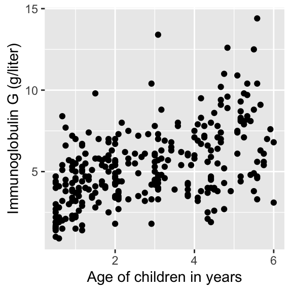
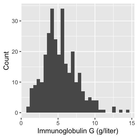
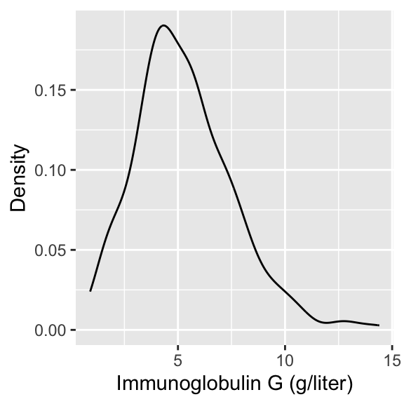
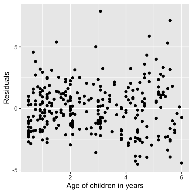
In today’s lecture, we will look at data on serum concentration (grams per litre) of immunoglobulin-G (IgG) in 298 children aged from 6 months to 6 years.
- A detailed discussion of this data set may be found in Isaacs et al. (1983) and Royston and Altman (1994).
For an example patient, we define $Y_{i}$ as the serum concentration value and $X_{i}$ as a child’s age, given in years.

Pulling the data

library(Brq)
data("ImmunogG")
head(ImmunogG)

  IgG Age
1 1.5 0.5
2 2.7 0.5
3 1.9 0.5
4 4.0 0.5
5 1.9 0.5
6 4.4 0.5

Visualizing IgG data

Modeling the association between age and IgG

Linear regression can be written as follows for $i = 1, \dots, n$ ,

$Y_{i} = α + β X_{i} + ϵ_{i}, ϵ_{i} \sim N (0, σ^{2}) .$

$β$ represent the change in IgG serum concentration with a one year increase in age.

Linear regression assumptions

$\begin{aligned} Y_{i} & = α + β X_{i} + ϵ_{i}, ϵ_{i} \sim N (0, σ^{2}) \\ = μ_{i} + ϵ_{i} . \end{aligned}$

Assumptions:

$Y_{i}$ are independent observations (independence).
$Y_{i}$ is linearly related to $X_{i}$ (linearity).
$ϵ_{i} = Y_{i} - μ_{i}$ is normally distributed (normality).
$ϵ_{i}$ has constant variance across $X_{i}$ (homoskedasticity).

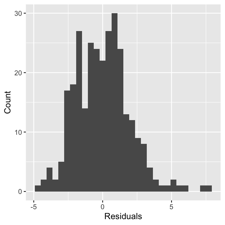
Assessing assumptions

Robust regression

Today we will learn about regression techniques that are robust to the assumptions of linear regression.
We will introduce the idea of robust regression by exploring ways to generalize the homoskedastic variance assumption in linear regression.
We will touch on heteroskedasticity, heavy-tailed distributions, and median regression (more generally quantile regression).

Why is robust regression not more comomon?

Despite their desirable properties, robust methods are not widely used. Why?
- Historically computationally complex.
- Not available in statistical software packages.
Bayesian modeling using Stan alleviates these bottlenecks!

Heteroskedasticity

Heteroskedasticity is the violation of the assumption of constant variance.
How can we handle this?
In OLS, there are approaches like heteroskedastic consistent errors, but this is not a generative model.
In the Bayesian framework, we generally like to write down generative models.

Modeling the scale with covariates

One option is to allow the sale to be modeled as a function of covariates.
It is common to model the log-transformation of the scale or variance to transform it to $R$ ,

$\log τ_{i} = z_{i} γ,$

where $z_{i} = (z_{i 1}, \dots, z_{i p})$ are a $p$ -dimensional vector of covariates and $γ$ are parameters that regress the covariates onto the log standard deviation.

Other options include: $\log τ_{i} = z_{i} γ + ν_{i}, ν_{i} \sim N (0, σ^{2})$
Other options include: $\log τ_{i} = f (μ_{i})$
Any plausible generative model can be specified!

Modeling the scale with covariates

data {
  int<lower = 1> n;
  int<lower = 1> p;
  int<lower = 1> q;
  vector[n] Y;
  matrix[n, p] X;
  matrix[n, q] Z;
}
parameters {
  real alpha;
  vector[p] beta;
  vector[q] gamma;
}
transformed parameters {
  vector[n] tau = exp(Z * gamma);
}
model {
  target += normal_lpdf(Y | alpha + X * beta, tau);
}

Heteroskedastic variance

We can write the regression model using a observation specific variance, $Y_{i} = α + x_{i} β + ϵ_{i}, ϵ_{i} \overset{i n d}{\sim} N (0, τ_{i}^{2}) .$
One way of writing the variance is: $τ_{i}^{2} = σ^{2} λ_{i}$ .
- $σ^{2}$ is a global scale parameter.
- $λ_{i}$ is an observation specific scale parameter.
In the Bayesian framework, we must place a prior on $λ_{i}$ .

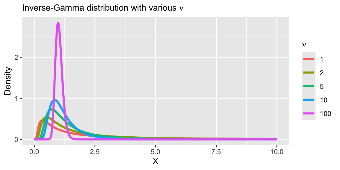
A prior to induce a heavy-tail

A common prior for $λ_{i}$ is as follows:

$λ_{i} \overset{i i d}{\sim} Inverse-Gamma (\frac{ν}{2}, \frac{ν}{2}) .$

A prior to induce a heavy-tail

A common prior for $λ_{i}$ is as follows:

$λ_{i} \overset{i i d}{\sim} Inverse-Gamma (\frac{ν}{2}, \frac{ν}{2}) .$

Under this prior, the marginal likelihood for $Y_{i}$ is equivalent to a Student-t distribution,

$Y_{i} = α + x_{i} β + ϵ_{i}, ϵ_{i} \overset{i i d}{\sim} t_{ν} (0, σ) .$

Understanding the equivalence

Heteroskedastic variances assumption is equivalent to assuming a heavy-tailed distribution.

$Y_{i} = α + x_{i} β + ϵ_{i}, ϵ_{i} \overset{i i d}{\sim} t_{ν} (0, σ) .$

$⟺$

$\begin{aligned} Y_{i} & = α + x_{i} β + ϵ_{i}, ϵ_{i} \overset{i n d}{\sim} N (0, σ^{2} λ_{i}) \\ λ_{i} & \overset{i i d}{\sim} Inverse-Gamma (\frac{ν}{2}, \frac{ν}{2}) \end{aligned}$

Note that since the number of $λ_{i}$ parameters is equal to the number of observations, this model will not have a proper posterior distribution without a proper prior distribution.

Understanding the equivalence

$\begin{aligned} f (Y_{i}) & = \int_{0}^{\infty} f (Y_{i}, λ_{i}) d λ_{i} \\ = \int_{0}^{\infty} f (Y_{i} | λ_{i}) f (λ_{i}) d λ_{i} \\ = \int_{0}^{\infty} N (Y_{i}; μ_{i}, σ^{2} λ_{i}) Inverse-Gamma (λ_{i}; \frac{ν}{2}, \frac{ν}{2}) d λ_{i} \\ = t_{ν} (μ_{i}, σ) . \end{aligned}$

The marginal likelihood can be viewed as a mixture of a Gaussian likelihood with an Inverse-Gamma scale parameter.

Understanding the equivalence

A random variable $T_{i} \overset{i i d}{\sim} t_{ν}$ can be written as a function of Gaussian and $χ^{2}$ random variables, $\begin{aligned} T_{i} & = \frac{Z_{i}}{\sqrt{\frac{W_{i}}{ν}}}, Z_{i} \overset{i i d}{\sim} N (0, 1), W_{i} \overset{i i d}{\sim} χ_{ν}^{2} \\ = \frac{Z_{i}}{\sqrt{\frac{1}{ν V_{i}}}}, V_{i} \overset{i i d}{\sim} Inv- χ_{ν}^{2}, V_{i} = W_{i}^{- 1} \\ = \sqrt{ν V_{i}} Z_{i}, λ_{i} = ν V_{i} \\ = \sqrt{λ_{i}} Z_{i}, λ_{i} \overset{i i d}{\sim} Inverse-Gamma (\frac{ν}{2}, \frac{ν}{2}) . \end{aligned}$

We then have: $Y_{i} = μ_{i} + σ T_{i} \sim t_{ν} (μ_{i}, σ) .$

Student-t in Stan

data {
  int<lower = 1> n;
  int<lower = 1> p;
  vector[n] Y;
  matrix[n, p] X;
}
parameters {
  real alpha;
  vector[p] beta;
  real<lower = 0> sigma;
  real<lower = 0> nu;
}
model {
  target += student_t_lpdf(Y | nu, alpha + X * beta, sigma);
}

Student-t in Stan: mixture

data {
  int<lower = 1> n;
  int<lower = 1> p;
  vector[n] Y;
  matrix[n, p] X;
}
parameters {
  real alpha;
  vector[p] beta;
  real<lower = 0> sigma;
  vector[n] lambda;
  real<lower = 0> nu;
}
transformed parameters {
  vector[n] tau = sigma * sqrt(lambda);
}
model {
  target += normal_lpdf(Y | alpha + X * beta, tau);
  target += inv_gamma_lpdf(lambda | 0.5 * nu, 0.5 * nu);
}

Why heavy-tailed distributions?

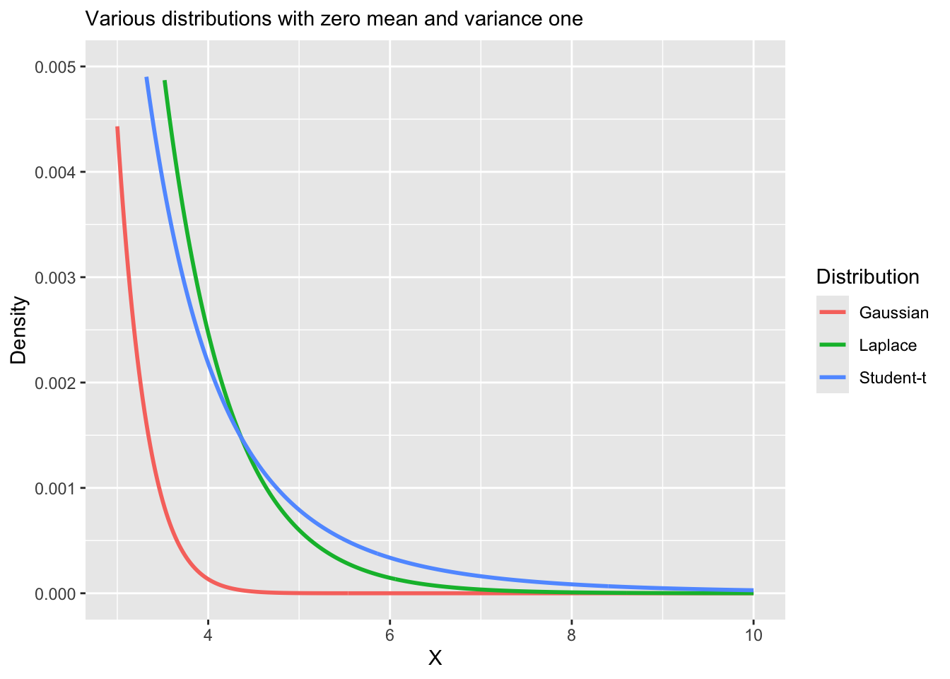
Replacing the normal distribution with a distribution with heavy-tails (e.g., Student-t, Laplace) is a common approach to robust regression.
Robust regression refers to regression methods which are less sensitive to outliers or small sample sizes.
Linear regression, including Bayesian regression with normally distributed errors is sensitive to outliers, because the normal distribution has narrow tail probabilities.
Our heteroskedastic model that we just explored is only one example of a robust regression model.

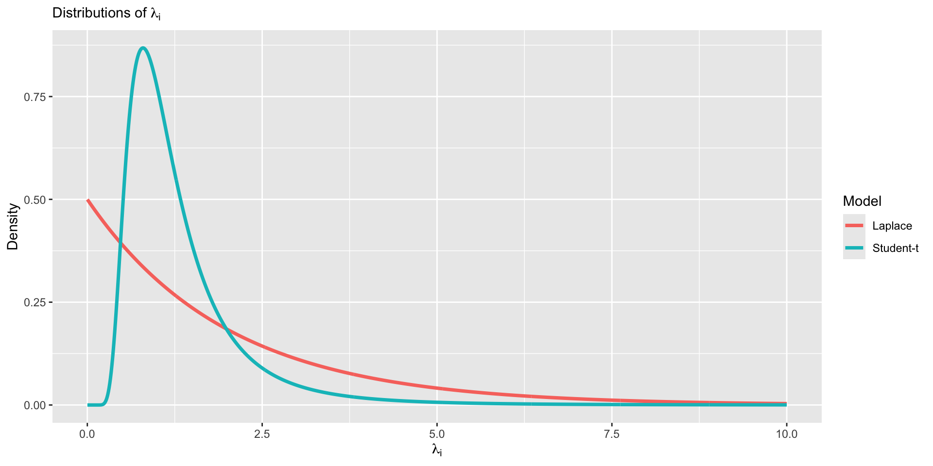
Vizualizing heavy tail distributions

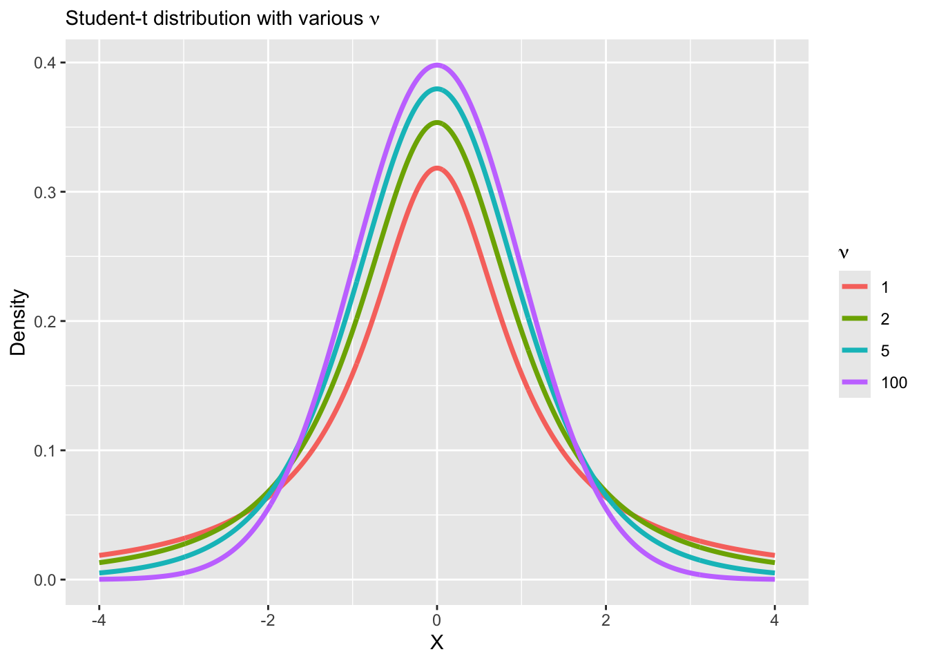
Vizualizing heavy tail distributions

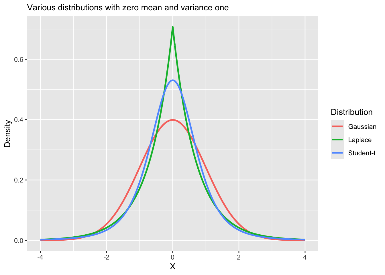
Vizualizing heavy tail distributions

Another example of robust regression

Let’s revisit our general heteroskedastic regression, $Y_{i} = α + x_{i} β + ϵ_{i}, ϵ_{i} \overset{i n d}{\sim} N (0, σ^{2} λ_{i}) .$
We can induce another form of robust regression using the following prior for $λ_{i}$ , $λ_{i} \sim Exponential (1 / 2)$ .

Another example of robust regression

Let’s revisit our general heteroskedastic regression, $Y_{i} = α + x_{i} β + ϵ_{i}, ϵ_{i} \overset{i n d}{\sim} N (0, σ^{2} λ_{i}) .$
We can induce another form of robust regression using the following prior for $λ_{i}$ , $λ_{i} \sim Exponential (1 / 2)$ .
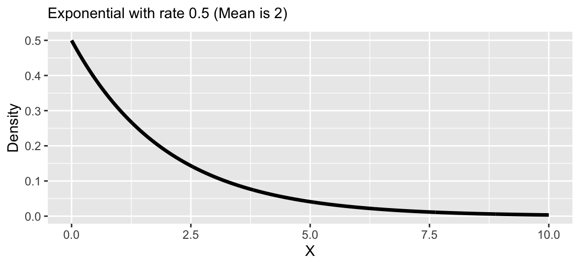
Under this prior, the induced marginal model is, $Y_{i} = α + x_{i} β + ϵ_{i}, ϵ_{i} \overset{i i d}{\sim} Laplace (μ = 0, σ) .$
This has a really nice interpretation!

Laplace distribution

Suppse a variable $Y_{i}$ follows a Laplace (or double exponential) distribution, then the pdf is given by,

$f (Y_{i} | μ, σ) = \frac{1}{2 σ} \exp {- \frac{| Y_{i} - μ |}{σ}}$

$E [Y_{i}] = μ$
$V (Y_{i}) = 2 σ^{2}$
Under the Laplace likelihood, estimation of $μ$ is equivalent to estimating the population median of $Y_{i}$ .

Median regression using Laplace

Least absolute deviation (LAD) regression minimizes the following objective function,

${\hat{α}}_{LAD}, {\hat{β}}_{LAD} = \arg min_{α, β} \sum_{i = 1}^{n} | Y_{i} - μ_{i} |, μ_{i} = α + x_{i} β .$

The Bayesian analog is the Laplace distribution,

$f (Y | α, β, σ) = {(\frac{1}{2 σ})}^{n} \exp {- \sum_{i = 1}^{n} \frac{| Y_{i} - μ_{i} |}{σ}} .$

Median regression using Laplace

The Laplace distribution is analogous to least absolute deviations because the kernel of the distribution is $| x - μ |$ , so minimizing the likelihood will also minimize the least absolute distances.
Laplace distribution is also known as the double-exponential distribution (symmetric exponential distributions around $μ$ with scale $σ$ ).
Thus, a linear regression with Laplace errors is analogous to a median regression,
Why is median regression considered more robust than regression of the mean?

Laplace regression in Stan

data {
  int<lower = 1> n;
  int<lower = 1> p;
  vector[n] Y;
  matrix[n, p] X;
}
parameters {
  real alpha;
  vector[p] beta;
  real<lower = 0> sigma;
}
model {
  target += double_exponential_lpdf(Y | alpha + X * beta, sigma);
}

Laplace regression in Stan: mixture

data {
  int<lower = 1> n;
  int<lower = 1> p;
  vector[n] Y;
  matrix[n, p] X;
}
parameters {
  real alpha;
  vector[p] beta;
  real<lower = 0> sigma;
  vector[n] lambda;
}
transformed parameters {
  vector[n] tau = sigma * sqrt(lambda);
}
model {
  target += normal_lpdf(Y | alpha + X * beta, tau);
  target += exponential_lpdf(lambda | 0.5);
}

Returning to IgG

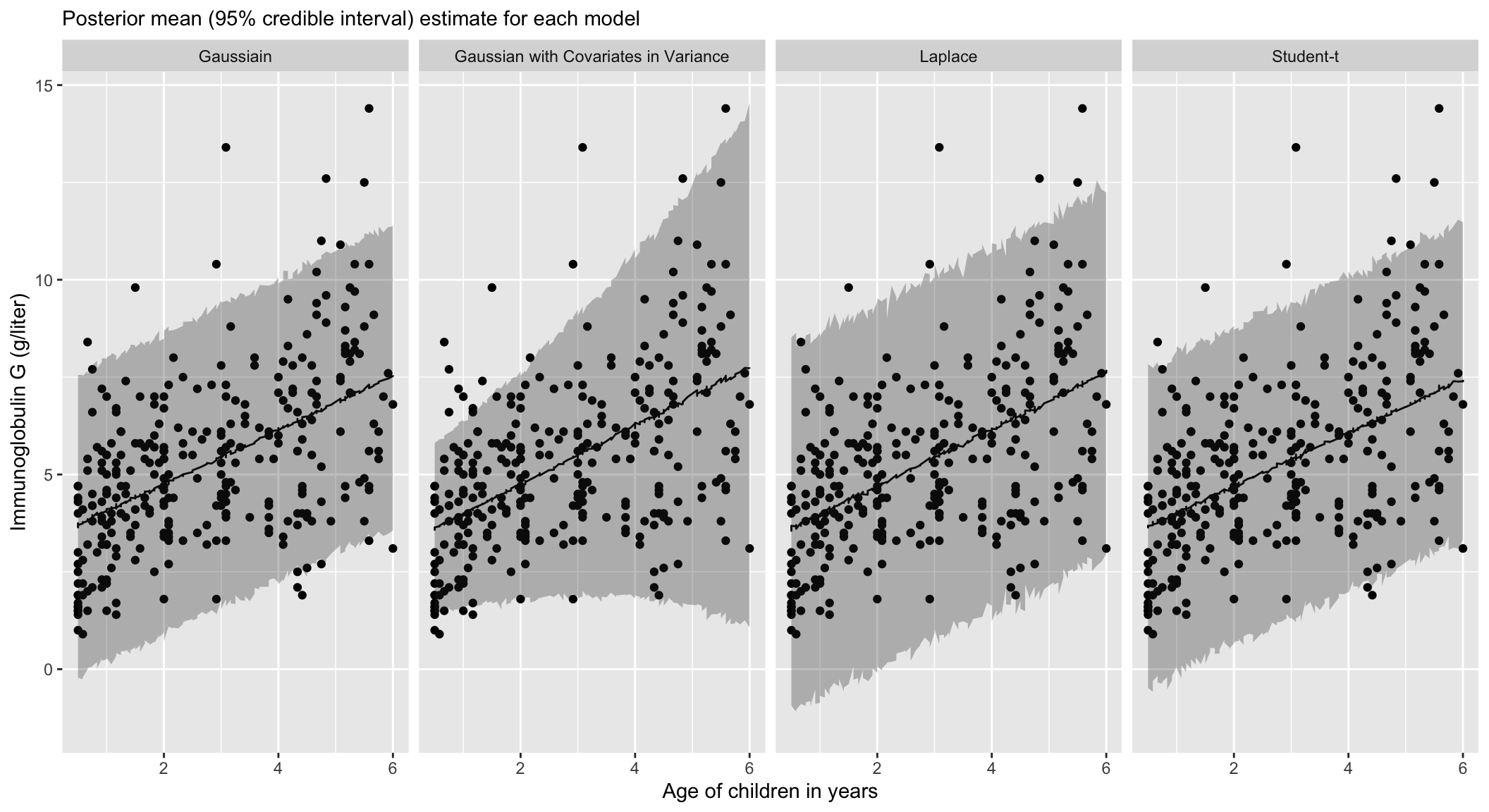
Posterior of $β$

Model	Mean	Lower	Upper
Laplace	0.73	0.56	0.89
Student-t	0.69	0.55	0.82
Gaussian	0.69	0.56	0.83
Gaussian with Covariates in Variance	0.76	0.62	0.89

Model Comparison

	elpd_diff	elpd_loo	looic
Student-t	0.00	-624.42	1248.84
Gaussian	-2.01	-626.43	1252.86
Gaussian with Covariates in Variance	-6.09	-630.51	1261.02
Laplace	-13.10	-637.52	1275.05

Examining the Student-t model fit

Inference for Stan model: anon_model.
4 chains, each with iter=2000; warmup=1000; thin=1; 
post-warmup draws per chain=1000, total post-warmup draws=4000.

        mean se_mean   sd 2.5% 97.5% n_eff Rhat
alpha   3.32    0.00 0.21 2.91  3.74  2084    1
beta[1] 0.69    0.00 0.07 0.55  0.82  2122    1
sigma   1.72    0.00 0.10 1.53  1.91  2744    1
nu      7.80    0.05 2.35 4.40 13.29  2617    1

Samples were drawn using NUTS(diag_e) at Sun Feb  9 14:54:53 2025.
For each parameter, n_eff is a crude measure of effective sample size,
and Rhat is the potential scale reduction factor on split chains (at 
convergence, Rhat=1).

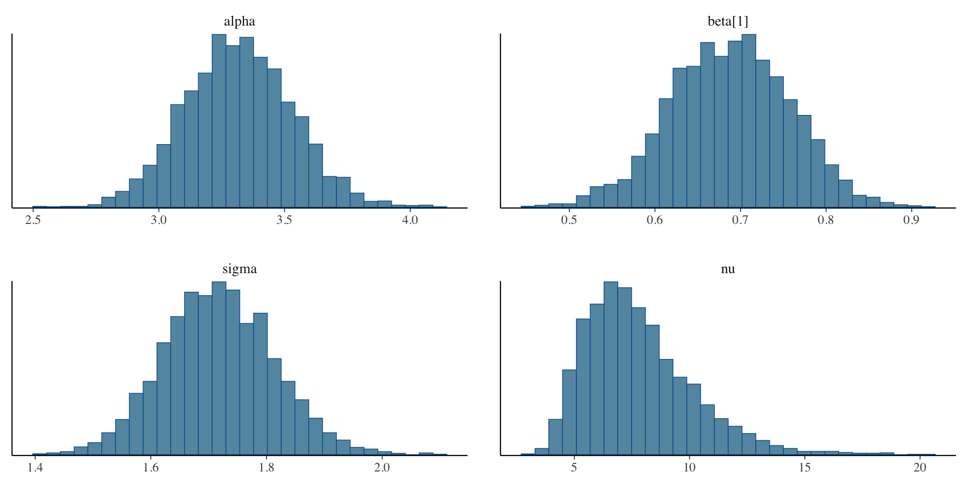
Examining the Student-t model fit

Summary of robust regression

Robust regression techniques can be used when the assumptions of constant variance and/or normality of the residuals do not hold.
Heteroskedastic variance can viewed as inducing extreme value distributions.
Extreme value regression using Student-t and Laplace distributions are robust to outliers.
Laplace regression is equivalent to median regression.

Prepare for next class

Work on HW 02, which is due before next class.
Complete reading to prepare for next Thursday’s lecture
Thursday’s lecture: Regularization