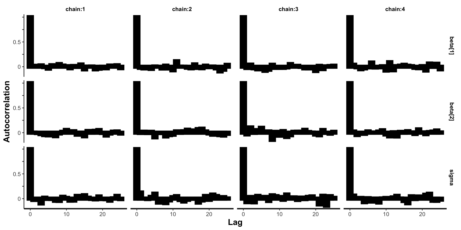
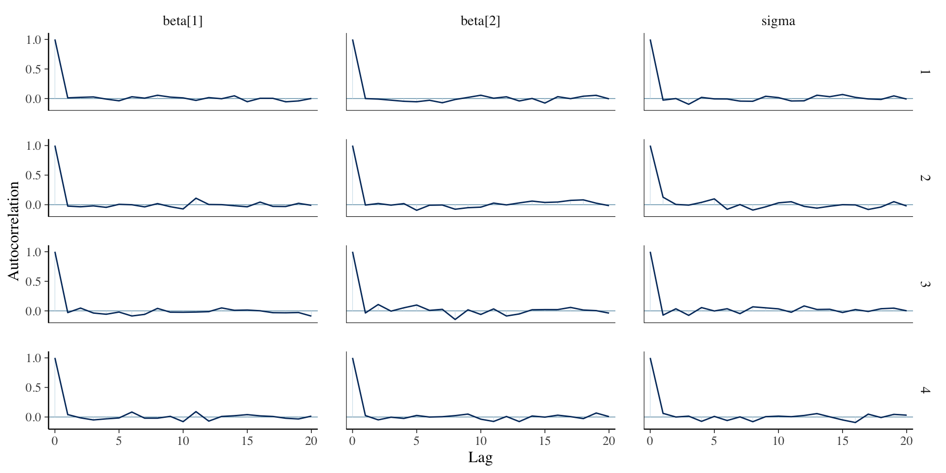
\[n_{eff}=ESS(\theta_i) = \frac{mS}{1 + 2 \sum_{h = 1}^{\infty} \rho (h)},\] where \(m\) is the number of chains, \(S\) is the number of MCMC samples, and \(\rho(h)\) is the \(h\)th order autocorrelation for \(\theta_i\).
The correlated MCMC sample of length \(mS\) has the same information as \(n_{eff}\) independent samples.
Rule of thumb: \(n_{eff}\) should be at least a thousand for all parameters.
Effective sample size for linear regression
print(fit, pars =c("beta", "sigma"))
Inference for Stan model: anon_model.
4 chains, each with iter=1000; warmup=500; thin=1;
post-warmup draws per chain=500, total post-warmup draws=2000.

         mean se_mean   sd  2.5%   25%   50%   75% 97.5% n_eff Rhat
beta[1] -1.48       0 0.16 -1.79 -1.58 -1.48 -1.37 -1.16  2002    1
beta[2]  3.30       0 0.15  3.01  3.19  3.29  3.40  3.59  1980    1
sigma    1.55       0 0.11  1.36  1.47  1.54  1.62  1.78  1909    1

Samples were drawn using NUTS(diag_e) at Fri Nov 22 10:44:51 2024.
For each parameter, n_eff is a crude measure of effective sample size,
and Rhat is the potential scale reduction factor on split chains (at
convergence, Rhat=1).
Standard errors of posterior mean estimates
The sample mean from our MCMC draws is a point estimate for the posterior mean.
The standard error (SE) of this estimate can be used as a diagnostic.
Assuming independence, the Monte Carlo standard error is \(\text{MCSE} = \frac{s}{\sqrt{S}},\) where \(s\) is the sample standard deviation and \(S\) is the number of samples.
A more realistic standard error is \(\text{MCSE} = \frac{s}{\sqrt{n_{eff}}}.\)
\(\text{MCSE} \rightarrow 0\) as \(S \rightarrow \infty\), whereas the standard deviation of the posterior draws approaches the standard deviation of the posterior distribution.
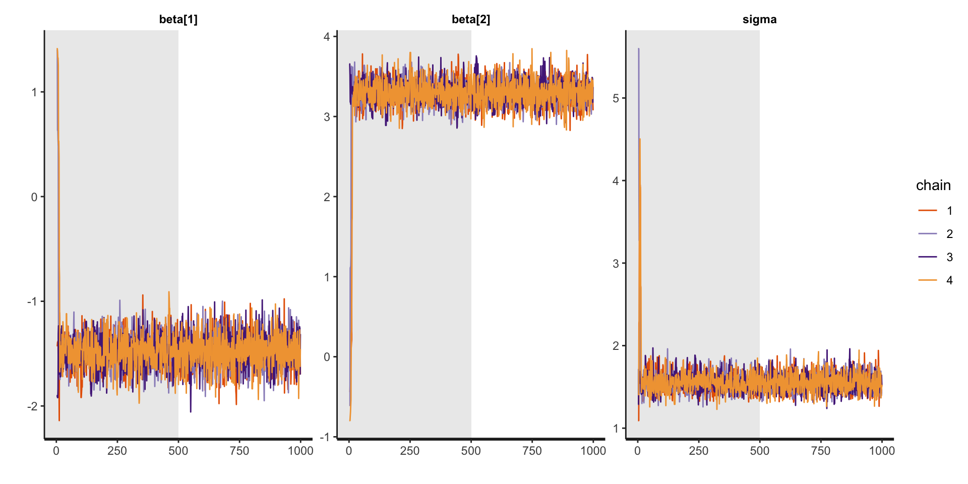
Assessing mixing using between- and within-sequence variances
For a scalar parameter, \(\theta\), define the MCMC samples as \(\theta_{ij}\) for chain \(j=1,\ldots,m\) and simulations \(i = 1,\ldots,n\). We can compute the between- and within-sequence variances:
The between-sequence variance, \(B\) contains a factor of \(n\) because it is based on the variance of the within-sequence means, \(\bar{\theta}_{\cdot j}\), each of which is an average of \(n\) values \(\theta_{ij}\).
Convergence metric: \(\widehat{R}\)
Estimate a total variance \(\mathbb{V}(\theta | \mathbf{Y})\) as a weighted mean of \(W\), \(B\)\[\widehat{\text{var}}^+(\theta | \mathbf{Y}) = \frac{n-1}{n}W + \frac{1}{n}B\]
This overestimates marginal posterior variance if starting points are overdispersed.
Given finite \(n\), \(W\) underestimates marginal posterior variance.
Single chains have not yet visited all points in the distribution.
When \(n \rightarrow \infty\), \(\mathbb{E}[W] \rightarrow \mathbb{V}(\theta | \mathbf{Y})\)
As \(\widehat{\text{var}}^+(\theta | \mathbf{Y})\) overestimates and \(W\) underestimates, we can compute
Inference for Stan model: anon_model.
4 chains, each with iter=1000; warmup=500; thin=1;
post-warmup draws per chain=500, total post-warmup draws=2000.

         mean se_mean   sd  2.5%   25%   50%   75% 97.5% n_eff Rhat
beta[1] -1.48       0 0.16 -1.79 -1.58 -1.48 -1.37 -1.16  2002    1
beta[2]  3.30       0 0.15  3.01  3.19  3.29  3.40  3.59  1980    1
sigma    1.55       0 0.11  1.36  1.47  1.54  1.62  1.78  1909    1

Samples were drawn using NUTS(diag_e) at Fri Nov 22 10:44:51 2024.
For each parameter, n_eff is a crude measure of effective sample size,
and Rhat is the potential scale reduction factor on split chains (at
convergence, Rhat=1).
A good rule of thumb is to want \(\widehat{R} \leq 1.1\).
What to do if your MCMC does not converge?
Gelman’s Folk Theorem:
When you have computational problems, often there’s a problem with your model.
Poor chain mixing is usually due to lack of parameter identification.
A parameter is identified if it has some unique effect on the data generating process that can be separated from the effect of the other parameters.
Solution: use simulated data where you know the true parameter values.
Informative as to whether the model is sufficient to estimate a parameter’s value.
Sampling issues: divergent iterations
You may get a warning in output from Stan with the number of iterations where the NUTS sampler has terminated prematurely.
Warning messages:1: There were 62 divergent transitions after warmup. Seehttps://mc-stan.org/misc/warnings.html#divergent-transitions-after-warmup2: There were 8 transitions after warmup that exceeded the maximum treedepth. Increase max_treedepth above 10. Seehttps://mc-stan.org/misc/warnings.html#maximum-treedepth-exceeded
Solution: If this warning appears, you can try:
Increase adapt_delta (double, between 0 and 1, defaults to 0.8).
Increase max_treedepth (integer, positive, defaults to 10).
Play with stepsize (double, positive, defaults to 1).
Sampling issues: divergent iterations
fit <-sampling(stan_model, data = stan_data, chains =4, iter =1000,control =list(adapt_delta =0.8, max_treedepth =10,stepsize =1))
See help(stan) for a full list of options that can be set in control.
Important: failing a resolution via the above go to http://mc-stan.org/ and do:
Look through manual for a solution.
Look through user forum for previous answers to similar problems.
Ask a question; be clear, and thorough - post as simple a model that replicates the issue.
Outside of this, you have an endless source of resources using Google/stackoverflow/stackexchange/ChatGPT. You can also post to Ed Discussion, go to office hours, and ask in lecture!
What to do when things go wrong: summary
Problems with sampling are almost invariably problems with the underlying model not the sampling algorithm.
Use fake data with all models to test for parameter identification (and that you’ve coded up correctly).
To debug a model that fails read error messages carefully, then try print statements.
Stan has an active developer and user forum, great documentation, and an extensive answer bank.
Posterior predictive checks
Posterior predictive checks
Last lecture we learned about posterior predictive distributions.
These can be used to check the model fit in our observed data.
The goal is to check how well our model can generate data that matches the observed data.
If our model is “good”, it should be able to generate new observations that resemble the observed data.
To perform the posterior predictive check, we must include the generated quantities code chunk.
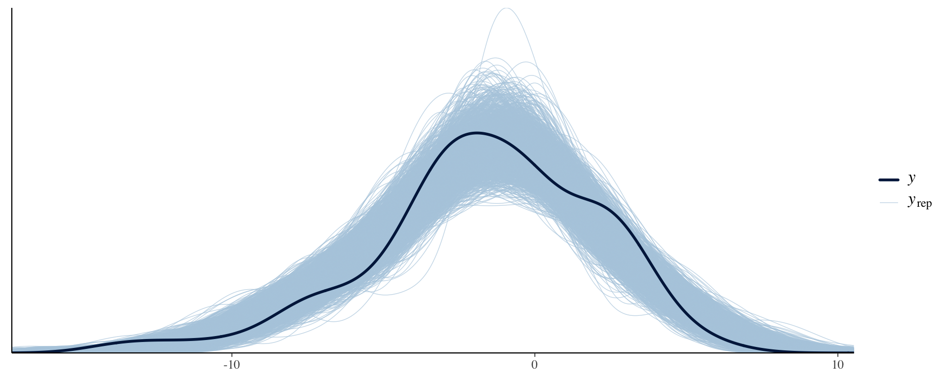
Comparing the PPD to the observed data distribution
library(rstan)library(bayesplot)Y_in_sample <-extract(fit, pars ="in_sample")$in_sampleppc_dens_overlay(Y, Y_in_sample)
PPD test statistics
The procedure for carrying out a posterior predictive check requires a test quantity, \(T(\mathbf{Y})\), for our observed data.
Suppose that we have samples from the posterior predictive distribution, \(\mathbf{Y}^{(s)} = \left\{Y_1^{(s)},\ldots,Y_n^{(s)}\right\}\) for \(s = 1,\ldots,S\).
We can compute: \(T\left(\mathbf{Y}^{(s)}\right) = \left\{T\left(Y_1^{(s)}\right),\ldots,\left(Y_n^{(s)}\right)\right\}\)
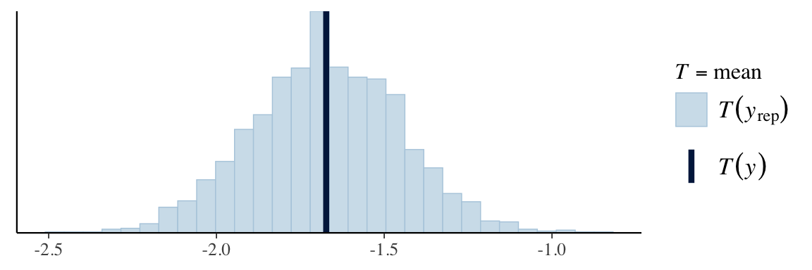
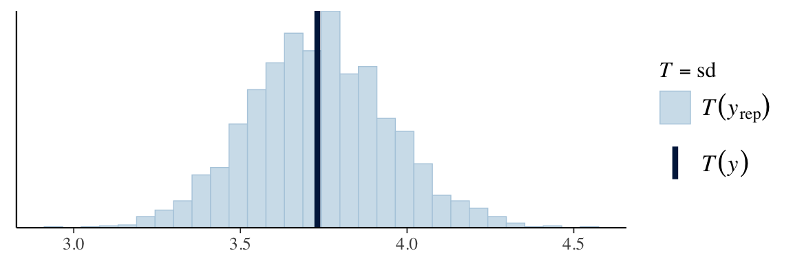
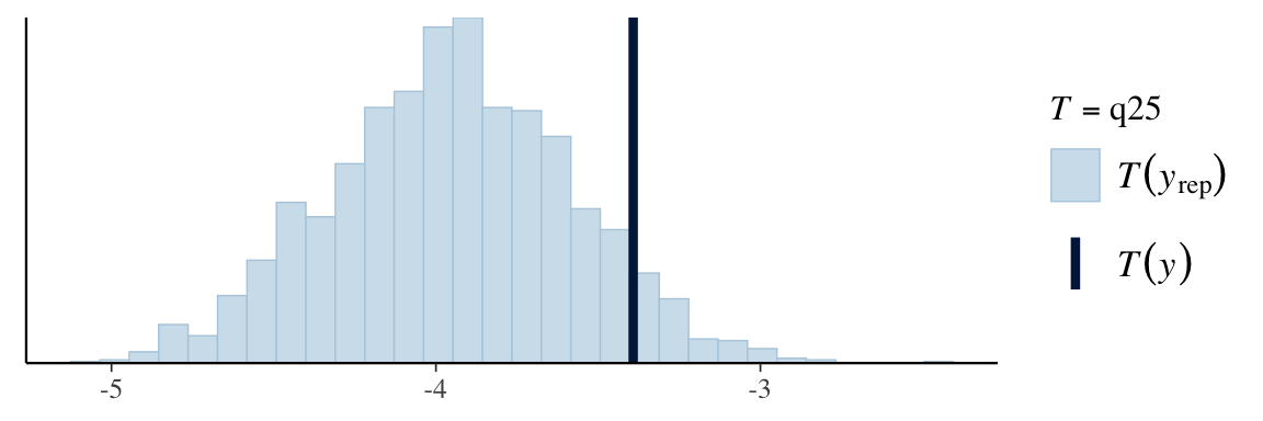
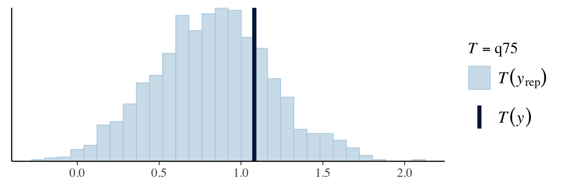
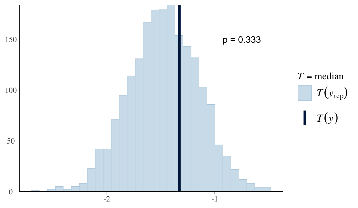
Our posterior predictive check will then compare the distribution of \(T\left(\mathbf{Y}^{(s)}\right)\) to the value from our observed data, \(T(\mathbf{Y})\).
\(T(\cdot)\) can be any statistics, including mean, median, etc.
When the predictive distribution is not consistent with the observed statistics it indicates poor model fit.
Visualizing posterior predictive check
ppc_stat(Y, Y_in_sample, stat ="mean") # from bayesplotppc_stat(Y, Y_in_sample, stat ="sd")q25 <-function(y) quantile(y, 0.25)q75 <-function(y) quantile(y, 0.75)ppc_stat(Y, Y_in_sample, stat ="q25")ppc_stat(Y, Y_in_sample, stat ="q75")
Posterior predictive p-values
plot <-ppc_stat(Y, Y_in_sample, stat ="median") # from bayesplotpvalue <-mean(apply(Y_in_sample, 1, median) >median(Y))plot +yaxis_text() +# just so I can see y-axis values for specifying them in annotate() below, but can remove this if you don't want the useless y-axis values displayed annotate("text", x =-0.75, y =150, label =paste("p =", pvalue))