Probabilistic Programming (Intro to Stan!)

Prof. Sam Berchuck

Jan 21, 2025

Review of last lecture

On Thursday, we performed posterior inference for Bayesian linear regression using Gibbs and Metropolis sampling.

• We obtained correlated samples from the posterior using MCMC.

• Gibbs required a lot math!

• Metropolis required tuning!

Today we will introduce Stan, a probabilistic programming language that uses Hamiltonian Monte Carlo to perform general Bayesian inference.

Learning objectives

By the end of this lecture you should:

• Know how to start coding up a model in Stan.

• Appreciate how easy Stan makes things for us compared to coding up the algorithm ourselves.

• Be able to fit a basic linear regression in Stan.

What is Stan and how do we use it?

• Stan is an intuitive yet sophisticated programming language that does the hard work for us.

• Programming language like R, Python, Matlab, C++…

• Works like most other languages: can use loops, conditional statements, and functions.

• Code up a model in Stan and then it implements HMC (actually something called NUTS) for us.

Why should we use Stan?

• Stan is the brainchild of Andrew Gelman at Colombia.

• Stan uses an extension of HMC called NUTS that automatically tunes. It is fast.

• Stan is simple to learn.

• Stan has excellent documentation (a manual full of extensive examples).

• Most important: Stan has a very active and helpful user forum and development team; for example, typical question answered in less than a couple of hours.

How do we use it?

Code up model in Stan code in a text editor and save as .stan file.

• Call Stan to run the model from:

  • R, python, the command line, Matlab, Stata, Julia

• Use one of the above to analyse the data (of course you can export to another one).

A straightforward example

Suppose:

• We record the height, \(Y_i\), of 10 people.

• We want a model to explain the variation, and choose a normal likelihood: \[Y_i \sim N(\mu, \sigma^2)\]

• We choose the following (independent) priors on each parameter:

  • \(\mu \sim N(0, 1)\)
  • \(\sigma^2 \sim IG(1, 1)\)

• Question: how do we code this up in Stan?

An example Stan program

data {
  real Y[10]; // height for 10 people
}
parameters {
  real mu;
  real<lower = 0> sigma2;
}
model {
  Y ~ normal(mu, sqrt(sigma2)); // likelihood
  mu ~ normal(0, 1); // prior for mu
  sigma2 ~ inv_gamma(1, 1); // prior for sigma
}

An example Stan program: data block

data {
  real Y[10]; // height for 10 people
}

• Declare all data that you will pass to Stan to estimate your model.

• Terminate all statements with a semi-colon ;.

• Use ## or // for comments.

An example Stan program: data block

data {
  real Y[10]; // height for 10 people
}

• We need to tell Stan the type of data variable. For example:

  • real for continuous data.

  • int for discrete data.

  • Arrays: above we specified Y as an array of continuous data of length 10.

An example Stan program: data block

data {
  real Y[10]; // height for 10 people
}

Can place limits on data, for example:

• real<lower = 0, upper = 1> X;

• real<lower = 0> Z;

Vectors and matrices; only contain reals and can be used for matrix operations.

real Y[10]; // array representation
vector[10] Y; // vector representation

An example Stan program: parameter block

parameters {
  real mu;
  real<lower = 0> sigma2;
}

• Declare all parameters that you use in your model.

• Place limits on variables, for example:

  • real<lower = 0> sigma2

A multitude of parameter types including some of the aforementioned:

• real for continuous parameters.

• Arrays of types, for example real beta[10]

An example Stan program: parameter block

parameters {
  real mu;
  real<lower = 0> sigma2;
}

• vector or matrix, specified by:

  • vector[5] beta

  • matrix[5, 3] gamma

• simplex for a parameter vector that must sum to 1.

• More exotic types like corr_matrix, or ordered.

An example Stan program: parameter block

parameters {
  real mu;
  real<lower = 0> sigma2;
}

Important: Stan is not developed yet to work with discrete parameters. Options for discrete parameters in Stan:

• Marginalize out the parameter. For example, suppose we have \(f(\boldsymbol{\beta}, \theta)\), where \(\boldsymbol{\beta}\) is continuous and \(\theta\) is discrete:

\(f(\boldsymbol{\beta}) = \sum_{i = 1}^K f(\boldsymbol{\beta}, \theta_i)\)

• Some models can be reformulated without discrete parameters.

An example Stan program: model block

model {
  Y ~ normal(mu, sqrt(sigma2)); // likelihood
  mu ~ normal(0, 1); // prior for mu
  sigma2 ~ inv_gamma(1, 1); // prior for sigma2
}

• Used to define:

  • Likelihood.

  • Priors on parameters.

If don’t specify priors on parameters Stan assumes you are using flat priors (which can be improper).

An example Stan program: model block

model {
  Y ~ normal(mu, sqrt(sigma2)); // likelihood
  mu ~ normal(0, 1); // prior for mu
  sigma2 ~ inv_gamma(1, 1); // prior for sigma2
}

Huge range of probability distributions covered, across a range of parameterizations. For example:

• Discrete: Bernoulli, binomial, Poisson, beta-binomial, negative-binomial, categorical, multinomial.

• Continuous unbounded: normal, skew-normal, student-t, Cauchy, logistic.

An example Stan program: model block

model {
  Y ~ normal(mu, sqrt(sigma2)); // likelihood
  mu ~ normal(0, 1); // prior for mu
  sigma2 ~ inv_gamma(1, 1); // prior for sigma2
}

• Continuous bounded: uniform, beta, log-normal, exponential, gamma, chi-squared, inverse-chi-squared, Weibull, Wiener diffusion, Pareto.

• Multivariate continuous: normal, student-t, Gaussian process.

• Exotics: Dirichlet, LKJ correlation distribution, Wishart and its inverse, Von-Mises.

Running Stan

Write model in a text editing program and save as a .stan file.

• To create a .stan file from RStudio, File -> New File -> Stan File.

###Load packages
library(rstan)

###Generate fake data
Y <- rnorm(10, mean = 0, sd = 1)

###Compile and run model, and save in fit
fit <- stan(file = 'straightforward.stan', data = list(Y = Y), 
            iter = 1000, chains = 4, seed = 1)

Running Stan on example model

###Compile and run model, and save in fit
fit <- stan(file = 'straightforward.stan', data = list(Y = Y), 
            iter = 1000, chains = 4, seed = 1)

The above R code runs NUTS for our model with the following options:

• \(S=1,000\) MCMC samples of which 500 are discarded as warm-up.

• Across 4 chains.

• Using a random number seed of 1 (good to ensure you can reproduce results).

Example model: results

###Print summary statistics
print(fit, probs = c(0.25, 0.5, 0.75))

Inference for Stan model: anon_model.
4 chains, each with iter=1000; warmup=500; thin=1; 
post-warmup draws per chain=500, total post-warmup draws=2000.

        mean se_mean   sd   25%   50%   75% n_eff Rhat
mu     -0.45    0.01 0.32 -0.66 -0.46 -0.26  1361    1
sigma2  1.23    0.02 0.62  0.81  1.09  1.48   865    1
lp__   -6.80    0.04 1.03 -7.21 -6.49 -6.06   808    1

Samples were drawn using NUTS(diag_e) at Tue Jan 21 14:36:33 2025.
For each parameter, n_eff is a crude measure of effective sample size,
and Rhat is the potential scale reduction factor on split chains (at 
convergence, Rhat=1).

Example model: results

###Extract posterior samples
pars <- extract(fit)
class(pars)

[1] "list"

names(pars)

[1] "mu"     "sigma2" "lp__"  

###Extract samples for particular parameters
pars <- extract(fit, pars = "mu")
class(pars$mu)

[1] "array"

dim(pars$mu)

[1] 2000

Visualize posterior

###Extract samples for particular parameters
library(ggplot2)
data.frame(mu = pars$mu) |>
  ggplot(aes(x = mu)) +
  geom_histogram() +
  labs(x = expression(mu), y = "Count", 
       subtitle = bquote("Posterior distribution for " ~ mu))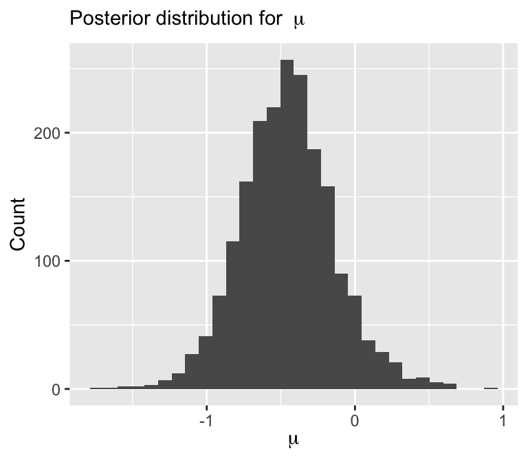

Quick note: what does \(\sim\) mean?

model {
  Y ~ normal(mu, sigma); // likelihood
  mu ~ normal(0, 1); // prior for mu
  sigma ~ inv_gamma(1, 1); // prior for sigma
}

• \(\sim\) doesn’t mean sampling, although often times it can be thought of as sampling

• MCMC/HMC makes use of the log-posterior

\[\log f(\boldsymbol{\theta} | \mathbf{Y}) \propto \log f(\boldsymbol{\theta}) + \sum_{i=1}^n \log f({Y}_i | \boldsymbol{\theta})\]

• As such \(\sim\) really means increment log probability

• All we have to do in Stan is specify the log-posterior!

Alternate way of specifying Stan models

model {
  target += normal_lpdf(Y | mu, sqrt(sigma2)); // likelihood
  target += normal_lpdf(mu | 0, 1); // prior for mu
  target += inv_gamma_lpdf(sigma2 | 1, 1); // prior for sigma
}

• target is a not a variable, but a special object that represents incremental log probability.

• target is initialized to zero.

• normal_lpdf is the log of the normal density of y given location mu and scale sigma:

• Stan documentation for normal distribution

target += std_normal_lpdf(mu) // prior for mu using standard normal

Linear regression using Stan: data and parameter chunks

data {
  int<lower = 1> n; // number of observations
  int<lower = 1> p; // number of covariates
  vector[n] Y; // outcome vector
  matrix[n, p + 1] X; // covariate vector
  real beta0; // location hyperparameter for beta
  real<lower = 0> sigma_beta; // scale hyperparameter for beta
  real<lower = 0> a; // shape hyperparameter for sigma2
  real<lower = 0> b; // scale hyperparameter for sigma2
}
parameters {
  vector[p + 1] beta;
  real<lower = 0> sigma2;
}

Linear regression using Stan: model chunk

model {
  for (i in 1:n) {
    target += normal_lpdf(Y[i] | X[i, ] * beta, sqrt(sigma2)); // likelihood
  }
  target += normal_lpdf(beta | beta0, sigma_beta); // prior for beta
  target += inv_gamma_lpdf(sigma2 | a, b); // prior for sigma2
}

Linear regression using Stan: vectorization

It is always a good idea to vectorize Stan code for faster and more efficient inference

model {
  target += normal_lpdf(Y | X * beta, sqrt(sigma2)); // likelihood
  target += normal_lpdf(beta | beta0, sigma_beta); // prior for beta
  target += inv_gamma_lpdf(sigma2 | a, b); // prior for sigma2
}

Linear regression using Stan

// saved in linear_regression.stan
data {
  int<lower = 1> n; // number of observations
  int<lower = 1> p; // number of covariates
  vector[n] Y; // outcome vector
  matrix[n, p + 1] X; // covariate vector
  real beta0; // location hyperparameter for beta
  real<lower = 0> sigma_beta; // scale hyperparameter for beta
  real<lower = 0> a; // shape hyperparameter for sigma2
  real<lower = 0> b; // scale hyperparameter for sigma2
}
parameters {
  vector[p + 1] beta;
  real<lower = 0> sigma2;
}
model {
  target += normal_lpdf(Y | X * beta, sqrt(sigma2)); // likelihood
  target += normal_lpdf(beta | beta0, sigma_beta); // prior for beta
  target += inv_gamma_lpdf(sigma2 | a, b); // prior for sigma2
}

Let’s simulate some data again

###True parameters
sigma <- 1.5 # true measurement error
beta <- matrix(c(-1.5, 3), ncol = 1) # true beta

###Simulation settings
n <- 100 # number of observations
p <- length(beta) - 1 # number of covariates

###Simulate data
set.seed(54) # set seed
X <- cbind(1, matrix(rnorm(n * p), ncol = p))
Y <- as.numeric(X %*% beta + rnorm(n, 0, sigma))

Fit linear regression using Stan

###Load packages
library(rstan)

###Create stan data object
stan_data <- list(n = n,
                  p = p,
                  Y = Y,
                  X = X,
                  beta0 = 0,
                  sigma_beta = 10,
                  a = 3, 
                  b = 1)
  
###Compile model separately
stan_model <- stan_model(file = "linear_regression.stan")

###Run model and save
fit <- sampling(stan_model, data = stan_data, 
                chains = 4, iter = 1000)
saveRDS(fit, file = "linear_regression_fit.rds")

Example model: results

###Print summary statistics
print(fit, probs = c(0.25, 0.5, 0.75))

Inference for Stan model: anon_model.
4 chains, each with iter=1000; warmup=500; thin=1; 
post-warmup draws per chain=500, total post-warmup draws=2000.

           mean se_mean   sd     25%     50%     75% n_eff Rhat
beta[1]   -1.48    0.00 0.15   -1.58   -1.48   -1.37  1951    1
beta[2]    3.30    0.00 0.15    3.20    3.30    3.40  1674    1
sigma2     2.35    0.01 0.33    2.12    2.32    2.55  1679    1
lp__    -196.98    0.04 1.29 -197.58 -196.63 -196.04   899    1

Samples were drawn using NUTS(diag_e) at Tue Jan 21 14:38:36 2025.
For each parameter, n_eff is a crude measure of effective sample size,
and Rhat is the potential scale reduction factor on split chains (at 
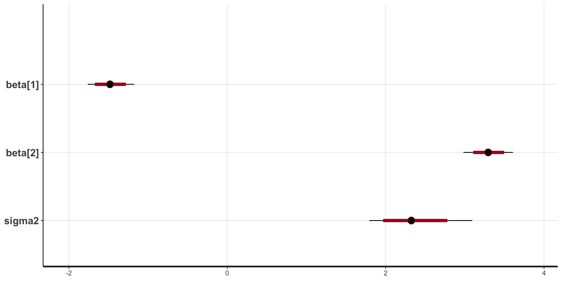
convergence, Rhat=1).

Stan plots: point estimate and intervals

stan_plot(fit, pars = c("beta", "sigma2"), include_warmup = FALSE,
          point_est = "median", ci_level = 0.8, outer_level = 0.95)

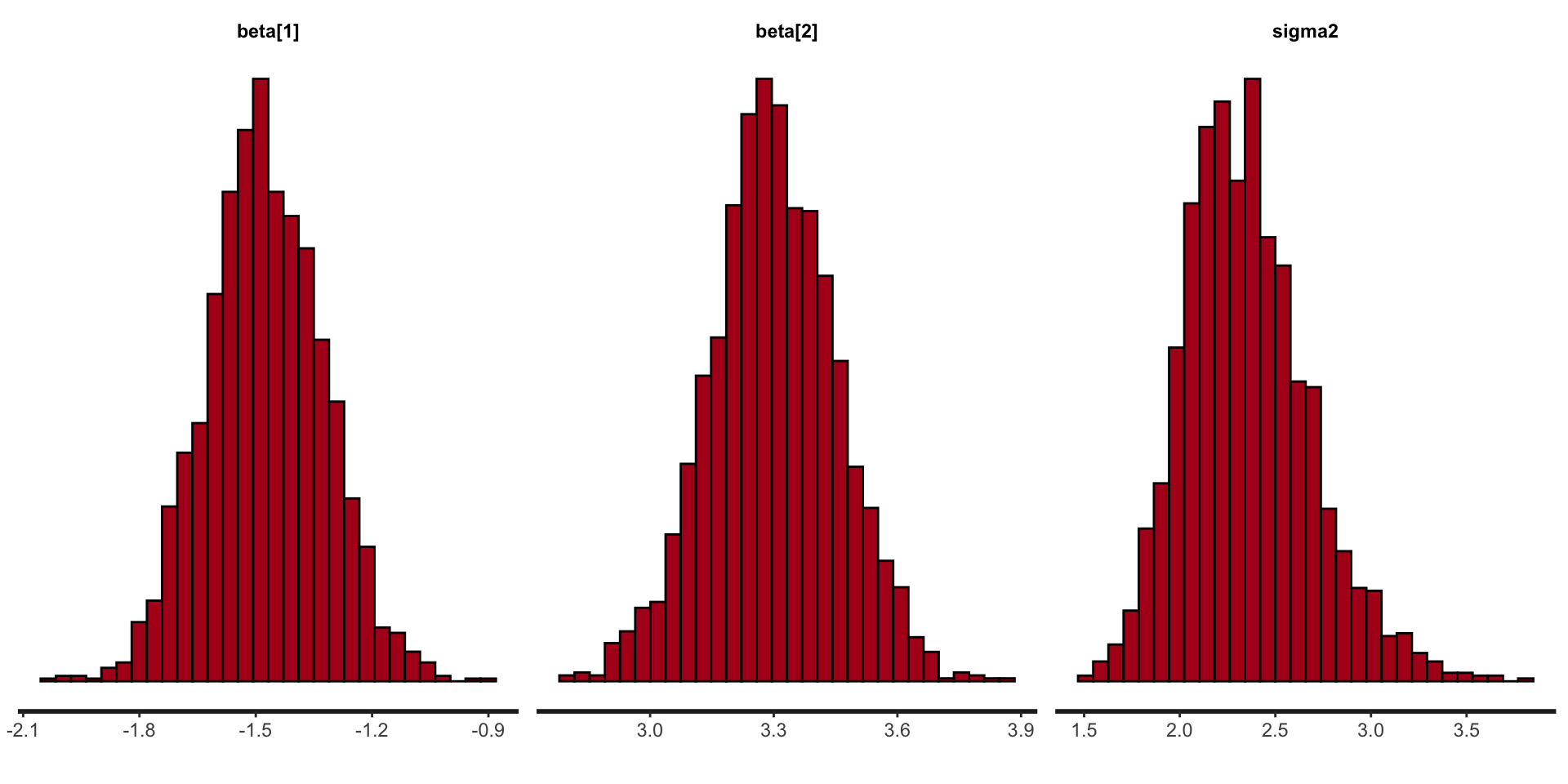
Stan plots: histogram

stan_hist(fit)

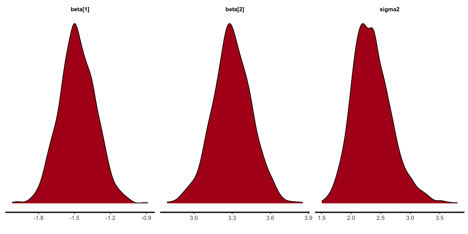
Stan plots: density

stan_dens(fit)

Stan: a few of the loops and conditions

Stan has pretty much the full range of language constructs to allow pretty much any model to be coded.

for (i in 1:10) {something;}

while (i > 1) {something;}

if (i > 1) {something 1;}
else if (i == 0) {something2;}
else {something 3;}

Stan speed concerns

While Stan is fast it pays to know the importance of each code block for efficiency.

• data: called once at beginning of execution.

• transformed data: called once at beginning of execution.

• parameters: every log probability evaluation!

• transformed parameters: every log probability evaluation!

• model: every log probability evaluation!

• generated quantities: once per sample.

• functions: how many times it is called depends on the function’s nature.

Stan in parallel

In R can run chains in parallel easily using:

library(rstan)
options(mc.cores = 8)

Stan summary

• Stan works by default with a HMC-like algorithm called NUTS.

• The Stan language is similar in nature to other common languages with loops, conditional statements and user-definable functions (didn’t cover here).

• Stan makes life easier for us than coding up the MCMC algorithms ourselves.

R packages that interface with Stan

• rstan, brms, cmdstanr, rstanarm

• rstan and cmdstanr you write the Stan code, which gives you the most options.

  • rstan has a more intuitive user interface.

  • cmdstanr is more memory efficient and a lightweight interface to Stan.

• rstanarm and brms you don’t need to write the Stan code yourself, which makes it easier to use Stan, but is limiting.

  • rstanarm’s biggest advantage is that the models are pre-compiled, but this is also it’s biggest limitation.

  • brms writes Stan code on the fly, so has many more models, some that are pretty advanced.

Prepare for next class

• Work on HW 01 which is due January 30

• Complete reading to prepare for next Thursday’s lecture

• Thursday’s lecture: Priors, Posteriors, and PPDs!