Monte Carlo Sampling

Prof. Sam Berchuck

Jan 14, 2025

Agenda

Monte Carlo (MC) sampling
Bayesian inference using MC sampling

Monte Carlo Sampling

Simulating \(\pi\) using Monte Carlo

Suppose we are interested in estimating \(\pi\).

We can formulate \(\pi\) as a function of the area of a square and circle.
Area of a circle: \(A_c = \pi r^2\)
Area of a square: \(A_s = 4 r^2\)
The ratio of the two areas is: \(\frac{A_c}{A_s} = \frac{\pi r^2}{4 r^2} \implies \pi = \frac{4 A_c}{A_s}\)

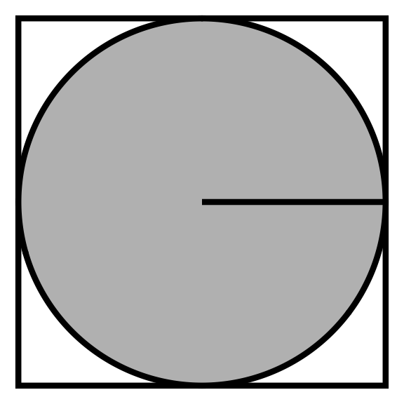
If we have an estimate for the ratio we can solve for \(\pi\). The challenge becomes estimating this ratio.

Monte Carlo sampling

We can take advantage of how quickly a computer can generate pseudo-random numbers.
There is a class of algorithms called Monte Carlo sampling that exploit randomness to estimate real world scenarios that would otherwise be difficult to explicitly calculate.
The name comes from the Monte Carlo Casino in Monaco, where the primary developer of the method, mathematician Stanislaw Ulam, was inspired by his uncle’s gambling habits. (This is who Stan was named after!)

Monte Carlo estimation of the ratio

We can use a Monte Carlo simulation to estimate the area ratio of the circle to the square.
Imagine you randomly drop grains of sand into the area of the square. By counting the total number of sand grains in the square (all of them since you’re an accurate dropper) to the number of sand grains inside the circle we get this estimate.
Multiply the estimated ratio by 4 and you get an estimate for \(\pi\).
The more grains of sand that are used the more accurate your estimate of \(\pi\).

Algorithm for estimating \(\pi\)

Generate a random point \((x, y)\) inside a square centered at the origin with length 2.

This is equivalent to assuming:

\(f_{X,Y}(x,y) = f_X(x)f_Y(y)\)
\(f_X(x) = Uniform(-1, 1)\), \(f_Y(y) = Uniform(-1, 1)\)

Determine whether the point falls inside the unit circle inscribed in the square by checking whether \(x^2 + y^2 \leq 1\).

Repeat steps 1 and 2 for a large number of points (\(S\)).

Algorithm for estimating \(\pi\)

Generate a random point \((x, y)\) inside a square centered at the origin with length 2.
Determine whether the point falls inside the unit circle inscribed in the square by checking whether \(x^2 + y^2 \leq 1\).
Repeat steps 1 and 2 for a large number of points (\(S\)).
Calculate the ratio of the number of points that fell inside the circle to the total number of points generated.

Multiply the ratio by 4 to estimate the value of \(\pi\).

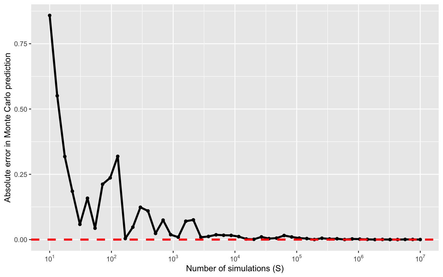
How big of a difference does \(S\) make

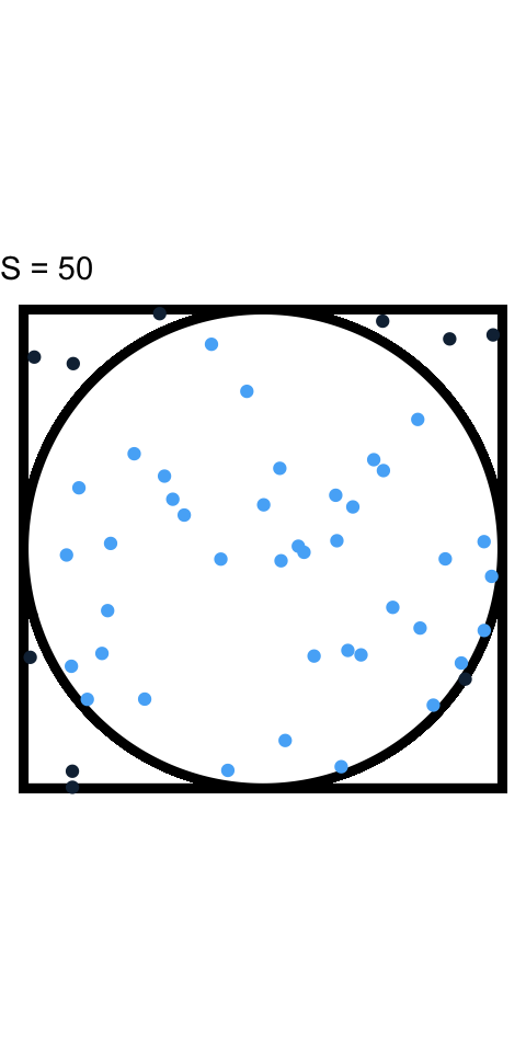
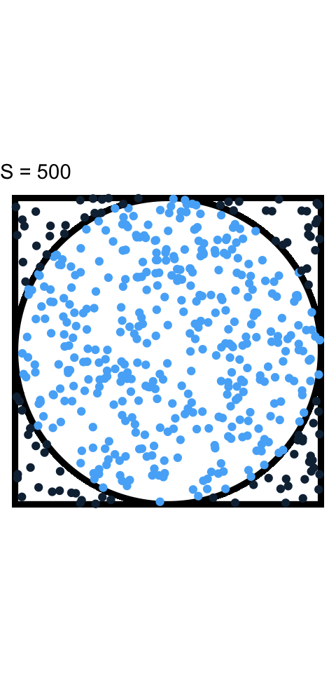
Estimating \(\pi\) with increasing \(S\)

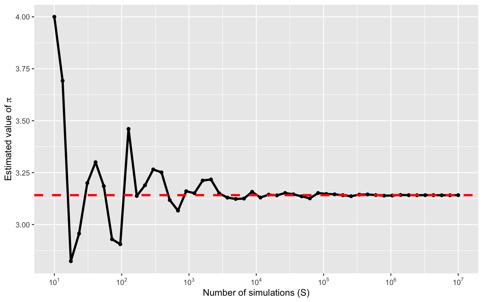
Error in estimating \(\pi\)

Intuition behing Monte Carlo sampling

Assume \(X \sim Uniform(-1,1)\) and \(Y \sim Uniform(-1,1)\).
We can write our problem as, \(\pi = 4P(X^2 + Y^2 \leq 1)\).
How could we do this without Monte Carlo?
Define, \(Z = X^2 + Y^2\). We could then use change-of-variables to compute the density of \(Z\) and then compute \(P(Z \leq 1)\).
- This is generally difficult!

Intuition behing Monte Carlo sampling

Instead, we could write our problem as an expectation and use the law of large numbers,

\[P(X^2 + Y^2 \leq 1) = \mathbb{E}_{X,Y}\left[1\left(X^2 + Y^2 \leq 1\right)\right].\]

Recall: \(\mathbb{E}_X[1(A)] = \int_A f_X(x)dx = P(X \in A)\).
We then have that, \[\frac{1}{S}\sum_{i = 1}^S 1\left(X_i^2 + Y_i^2 \leq 1\right) \rightarrow \mathbb{E}_{X,Y}\left[1\left(X^2 + Y^2 \leq 1\right)\right],\]

where \((X_i,Y_i) \sim f(X,Y)\).

Bayesian inference using MC sampling

Computing a Bayesian posterior
Posterior inference using MC sampling

A motivating example

Suppose we are interested in estimating the prevalence of diabetes in Durham County. We aim to estimate this prevalence by taking a sample of \(n\) individuals in Durham County and we record whether or not they have diabetes, \(Y_i\).
We assume that \(Z = \sum_{i=1}^n Y_i \sim Binomial(n, \pi)\) for \(i = 1,\ldots,n\).
Our goal is to estimate \(\pi\) and perform statistical inference (e.g., point estimation, interval estimation, etc.).

Posterior inference

In Bayesian statistics, inference is encoded through the posterior distribution,

\[\begin{aligned} f(\pi | Z) &= \frac{f(Z | \pi)f(\pi)}{f(Z)},\\ &= \frac{f(Z | \pi)f(\pi)}{\int f(Z | \pi)f(\pi)d\pi}. \end{aligned}\]

All we have to do is specify the likelihood and prior.

Likelihood specification

\(Z\) is a Binomial distribution with pmf,

\[f(Z | \pi) = P(Z = z) = {n \choose z} \pi^z(1-\pi)^{n-z},\]

where \(z \in \{0, 1, \ldots, n\}\).

\({n \choose z} = \frac{n!}{z!(n-z)!} = \frac{\Gamma(n+1)}{\Gamma(z+1)\Gamma(n-z+1)}\)
\(\Gamma(x) = (x-1)!\)

Prior specification

What do we know about \(\pi\)?

\(\pi\) is continuous.
\(\pi \in (0,1)\).

We should place a distribution on \(\pi\) that permits these properties.

One option is the Beta distribution, \(\pi \sim Beta(\alpha,\beta)\), \[f(\pi) = \frac{\Gamma(\alpha)\Gamma(\beta)}{\Gamma(\alpha+\beta)}\pi^{\alpha-1}(1-\pi)^{\beta-1}.\]

Computing the marginal likelihood

Under our prior specification, we can compute the marginal likelihood, \(f(Z)\):

\[\begin{aligned} f(Z) &= \int f(Z | \pi) f(\pi) d\pi\\ &= \int {n \choose z} \pi^z(1-\pi)^{n-z} \frac{\Gamma(\alpha)\Gamma(\beta)}{\Gamma(\alpha+\beta)}\pi^{\alpha-1}(1-\pi)^{\beta-1} d\pi\\ &= {n \choose z}\frac{\Gamma(\alpha)\Gamma(\beta)}{\Gamma(\alpha+\beta)} \int \underbrace{\pi^{(\alpha + z) - 1}(1-\pi)^{(\beta + n - z) - 1}}_{Beta\text{ }kernel} d\pi \end{aligned}\]

Definition

The part of the pdf/pmf that depends on the variable is called the kernel.

Example: The kernel of the Beta pdf is \(\pi^{\alpha-1}(1-\pi)^{\beta-1}\)

Computing the marginal likelihood

Under our prior specification, we can compute the marginal likelihood, \(f(Z)\):

\[\begin{aligned} f(Z) &= {n \choose z}\frac{\Gamma(\alpha)\Gamma(\beta)}{\Gamma(\alpha+\beta)} \int \pi^{(\alpha + z) - 1}(1-\pi)^{(\beta + n - z) - 1} d\pi\\ &= {n \choose z}\frac{\Gamma(\alpha)\Gamma(\beta)}{\Gamma(\alpha+\beta)} \frac{\Gamma(\alpha+\beta + n)}{\Gamma(\alpha + z)\Gamma(\beta + n - z)}. \end{aligned}\]

We can then compute the posterior

\[\begin{aligned} f(\pi | Z) &= \frac{f(Z | \pi) f(\pi)}{f(Z)}\\ &= \frac{{n \choose z} \pi^z(1-\pi)^{n-z} \times \frac{\Gamma(\alpha)\Gamma(\beta)}{\Gamma(\alpha+\beta)}\pi^{\alpha-1}(1-\pi)^{\beta-1}}{{n \choose z}\frac{\Gamma(\alpha)\Gamma(\beta)}{\Gamma(\alpha+\beta)} \frac{\Gamma(\alpha+\beta) }{\Gamma(\alpha + z)\Gamma(\beta + n - z)}}\\ &=\frac{\Gamma(\alpha+z)\Gamma(\beta+n-z)}{\Gamma(\alpha + \beta + n)}\pi^{(\alpha + z) - 1} (1 - \pi)^{(\beta + n - z) - 1}\\ &=Beta\left(\alpha + z, \beta + n - z\right). \end{aligned}\]

A prior that is considered conjugate yields a posterior with the same distribution.
The Beta distribution is conjugate for the Bernoulli/Binomial distributions.

Computing the posterior

In general, computing the marginal likelihood, \(f(Z)\), is extremely difficulty.
An easier approach is to use the kernel trick.

\[\begin{aligned} f(\pi | Z) &\propto f(Z | \pi) f(\pi)\\ &\propto \pi^z (1-\pi)^{n - z} \pi^{\alpha-1}(1-\pi)^{\beta-1} \\ &= \pi^{\left(\alpha + z\right) - 1} (1-\pi)^{\left(\beta + n - z\right) - 1}\\ &= Beta\left(\alpha + z, \beta + n - z\right). \end{aligned}\]

This only works when a conjugate prior is used.

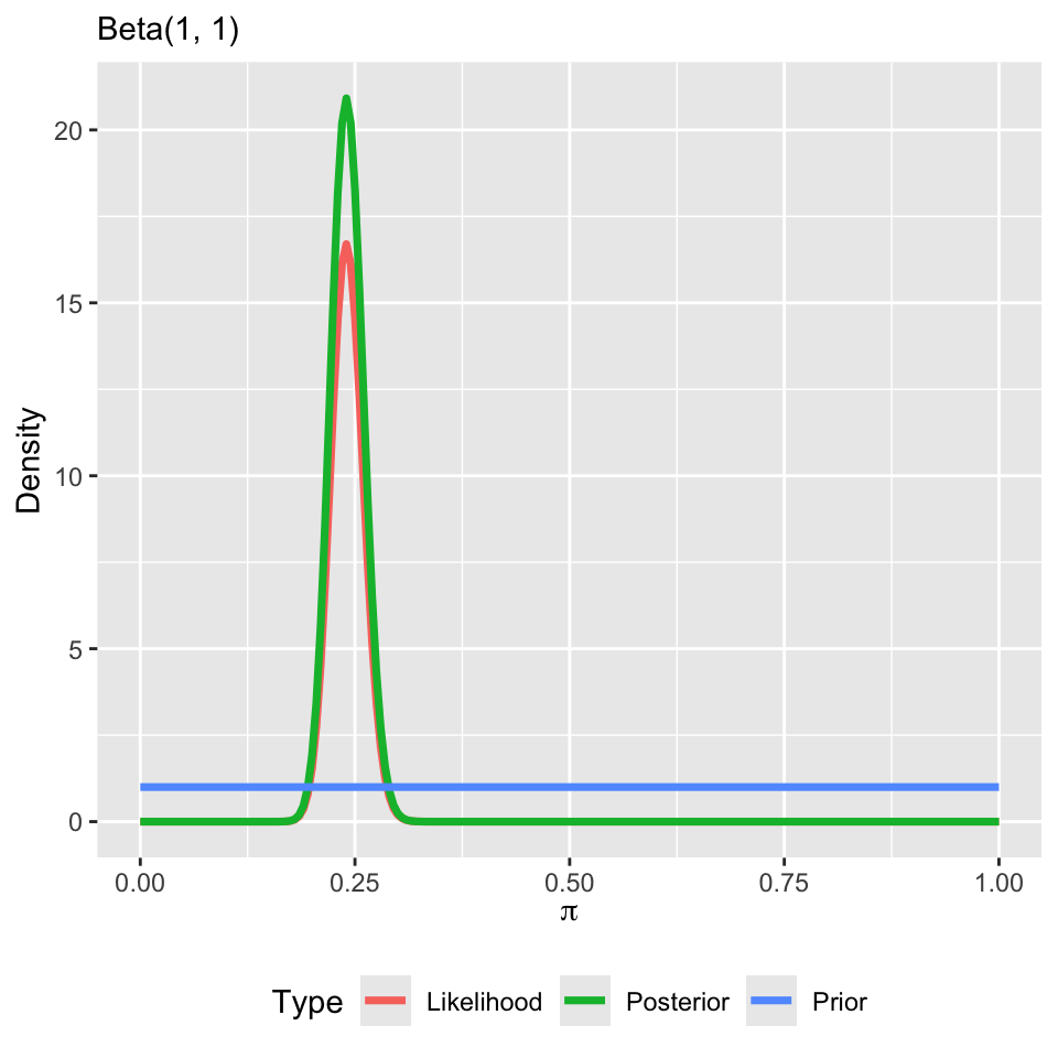
Let’s inspect the posterior

Suppose we conducted a simple random sample of 500 individuals in Durham County and 120 responsed that they had diabetes and 380 that they did not.
The posterior becomes, \(Beta\left(\alpha + 120, \beta + 380\right)\).
We must choose our prior distribution wisely.
Note that:
- \(\mathbb{E}[\pi] = \alpha/(\alpha + \beta)\)
- \(\mathbb{V}(\pi) = (\alpha\beta)/[(\alpha + \beta)^2(\alpha + \beta + 1)]\).
Typically, \(\alpha = \beta = 1\), which corresponds to a uniform prior on \(\pi\).

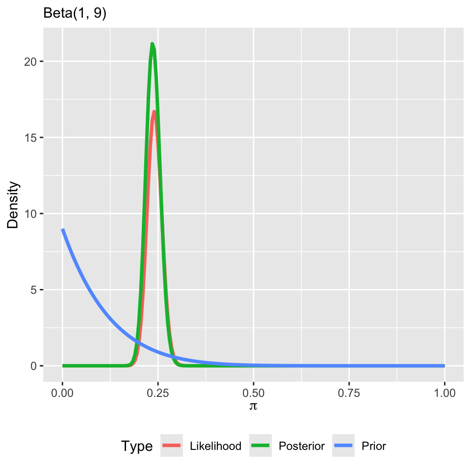
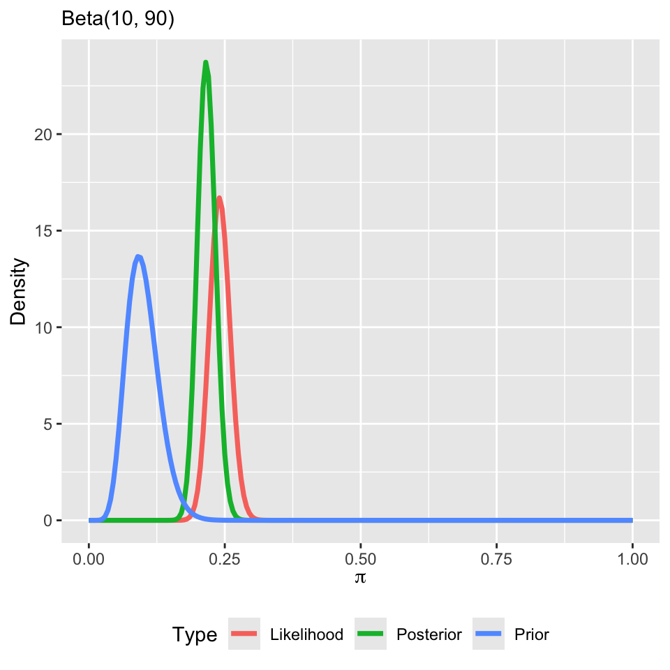
Let’s inspect the posterior

Suppose my prior changes

Summarizing the posterior

We now have a posterior distribution. What do we do now?

Posterior means, medians, modes, and variances

Joint, conditional, and marginal probabilities, for example: \(P(\pi < c | Z)\)

\(\alpha\)-quantiles: \(\{q_{\alpha} : P(\pi < q_{\alpha} | Z) = \alpha\}, \alpha \in (0,1)\)

\(\ldots\)

How do we go about computing these summaries?

Summarization can be complex

Posteriors are often not available in closed form.
Even when we have a closed form posterior, it can be difficult to compute summaries of interest.
For example, consider \(P(\pi < c | Z)\). What are our options to calculate this probability?
- Direct integration (by hand)
- Numerical integration/software packages (e.g., \(\texttt{pbeta}\))

These methods work well for standard posterior quantities and distributions.

Summarizing the posterior

However, sometimes we will want to summarize other aspects of a posterior distribution.

\(P(\pi \in A| Z)\) for some arbitrary set \(A\)
Means and standard deviations of some function of \(\pi\), \(g\left(\pi\right)\)
The posterior distribution of functions of many parameters:
- \(|\pi_1 - \pi_2|\), \(\pi_1/\pi_2\), \(\max\left\{\pi_1,\ldots,\pi_p\right\}\), \(\dots\)
Obtaining exact values for these posterior quantities can be difficult or even impossible.

What are our options?

Monte Carlo sampling

Monte Carlo (MC) sampling

Integration method based on random sampling
The general principles and procedures remain relatively constant across a broad class of problems
Suppose we have \(S\) iid samples from our posterior distribution: \(\pi^{\left(1\right)},\ldots,\pi^{\left(S\right)}\stackrel{\text{iid}}{\sim}f\left(\pi|\mathbf{Y}\right)\)
Then the empirical distribution of \(\left\{\pi^{\left(1\right)},\ldots,\pi^{\left(S\right)}\right\}\) would approximate \(f\left(\pi|\mathbf{Y}\right)\), with the approximation improving as \(S\) increases
The empirical distribution of \(\left\{\pi^{\left(1\right)},\ldots,\pi^{\left(S\right)}\right\}\) is known as a MC approximation to \(f\left(\pi|\mathbf{Y}\right)\)

MC approximation

Let \(g\left(\pi\right)\) be (just about) any function of \(\pi\). The law of large numbers says that if,

\[\pi^{\left(1\right)},\ldots,\pi^{\left(S\right)}\stackrel{\text{iid}}{\sim}f\left(\pi|\mathbf{Y}\right),\] then, \[\frac{1}{S}\sum_{s=1}^S g\left(\pi^{\left(s\right)}\right)\rightarrow \mathbb{E}\left[g\left(\pi\right)|\mathbf{Y}\right]=\int g\left(\pi\right)f\left(\pi|\mathbf{Y}\right)d\pi,\] as \(S\rightarrow \infty\).

MC approximation

Implications (as \(S\rightarrow \infty\)):
- \(\overline{\pi}=\frac{1}{S}\sum_{s=1}^S \pi^{\left(s\right)} \rightarrow \mathbb{E}\left[\pi|\mathbf{Y}\right]\)
- \(\frac{1}{S-1}\sum_{s=1}^S \left(\pi^{\left(s\right)}-\overline{\pi}\right)^2 \rightarrow \mathbb{V}\left(\pi|\mathbf{Y}\right)\)
- \(\frac{1}{S}\sum_{s=1}^S 1\left(\pi^{\left(s\right)}\leq \mathbf{c}\right) \rightarrow P\left(\pi\leq \mathbf{c} | \mathbf{Y}\right)\)
- \(\alpha\)-quantile of \(\left\{\pi^{\left(1\right)},\ldots,\pi^{\left(S\right)}\right\}\rightarrow q_{\alpha}\)
Just about any aspect of the posterior distribution can be approximated arbitrarily exactly with a large enough MC sample

Posterior inference for arbitrary functions

Interest in the posterior distribution of a function of \(\pi\), \(g\left(\pi\right)\)

MC sampling plan:
- Draw \(\pi^{\left(1\right)}\) from \(f\left(\pi|\mathbf{Y}\right)\), calculate \(g\left(\pi^{\left(1\right)}\right)\)
  
  \(\ldots\)
- Draw \(\pi^{\left(S\right)}\) from \(f\left(\pi|\mathbf{Y}\right)\), calculate \(g\left(\pi^{\left(S\right)}\right)\)
\(\Rightarrow g\left(\pi^{\left(1\right)}\right),\ldots,g\left(\pi^{\left(S\right)}\right)\stackrel{\text{iid}}{\sim}f\left(g\left(\pi\right)|\mathbf{Y}\right)\)
Therefore, similar quantities can be estimated (posterior mean, variance, quantiles, distribution, etc.)

How many samples to take?

We can use a central limit theorem: \(\sqrt{S}\left(\overline{\pi}-\mathbb{E}[\pi | \mathbf{Y}]\right)/\sigma \stackrel{d}{\rightarrow} \text{N}\left(0,1\right)\),

\(\overline{\pi}=\frac{1}{S}\sum_{s=1}^S \pi^{\left(s\right)}\)
\(\sigma^2 = \mathbb{V}\left(\overline{\pi}\right) = \frac{1}{S^2}\sum_{s=1}^S\mathbb{V}\left(\pi^{(s)}\right) = \frac{1}{S}\mathbb{V}\left(\pi | \mathbf{Y}\right)\).

\(\implies \overline{\pi}\approx N\left(\mathbb{E}[\pi | \mathbf{Y}],\sigma^2/S\right)\)

MC standard error: \(\sqrt{\frac{\widehat{\sigma}^2}{S}}\), \(\widehat{\sigma}^2=\frac{1}{S-1}\sum_{s=1}^S\left(\pi^{\left(s\right)}-\overline{\pi}\right)^2\)

Approximate 95% MC confidence interval for the posterior mean: \(\overline{\pi} \pm 2\sqrt{\frac{\widehat{\sigma}^2}{S}}\)

Choose \(S\) large enough to report the posterior mean with your desired precision
Reporting MC standard errors for the posterior mean is a good way to indicate that \(S\) is large enough

Returning to our posterior

Let’s obtain \(S = 1,000\) samples from our posterior.

pi_samples <- rbeta(1000, 1 + 120, 1 + 380)

We can compute the posterior mean and variance.

mean(pi_samples)

[1] 0.2404674

var(pi_samples)

[1] 0.0003437017

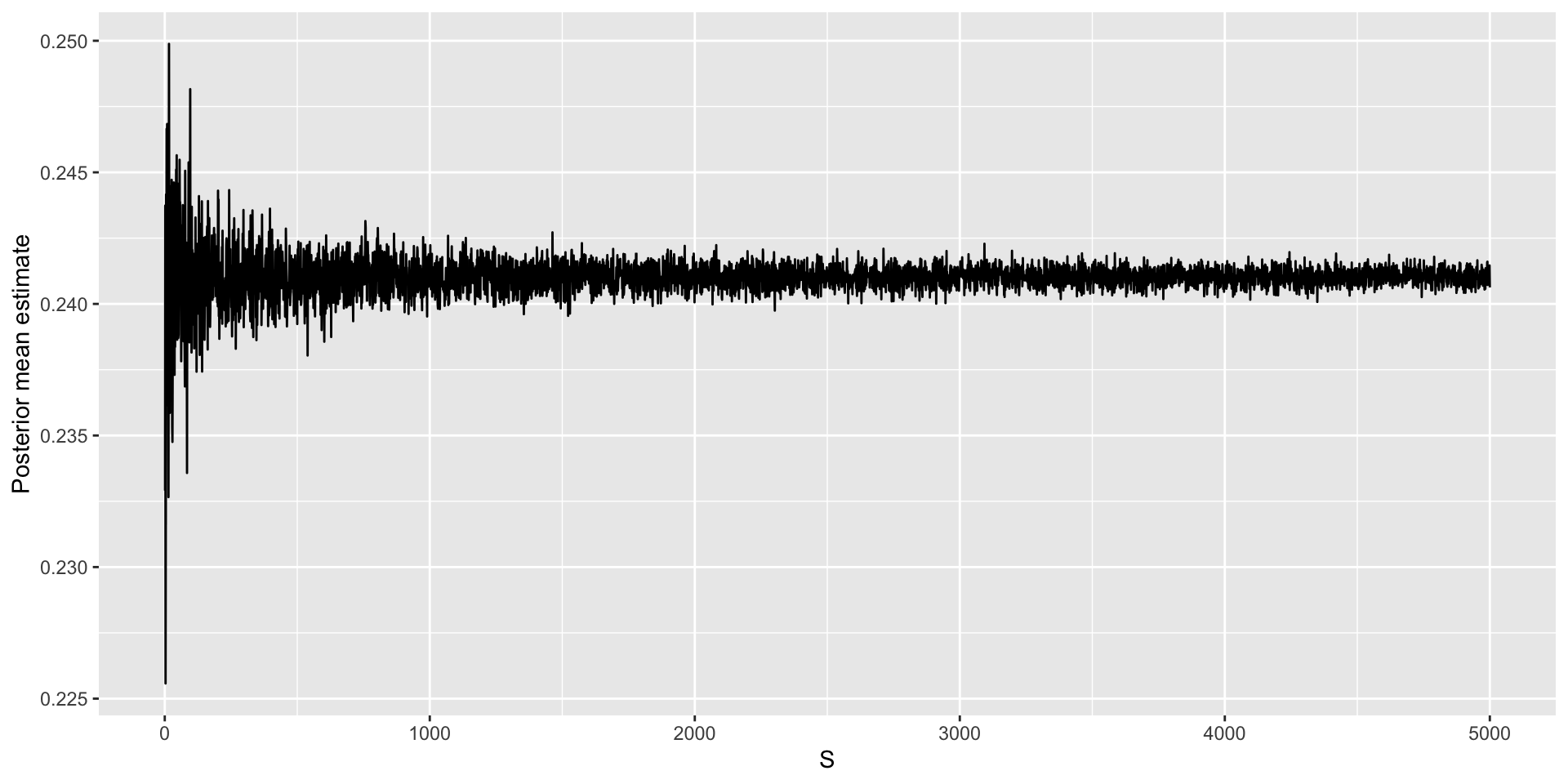
Assessing accuracy

Additional posterior summaries

# median
median(pi_samples)

[1] 0.2402345

# 95% credible intervals
quantile(pi_samples, probs = c(0.025, 0.975))

     2.5%     97.5% 
0.2035750 0.2784977

# evaluating probability
mean(pi_samples < 0.25)

[1] 0.6992

# summarizing arbitrary functions of the parameters
pi_new <- pi_samples^3 - pi_samples
c(mean(pi_new), quantile(pi_new, probs = c(0.025, 0.975)))

                 2.5%      97.5% 
-0.2264329 -0.2568972 -0.1951383

Additional examples of MC sampling

Poisson random variable

Suppose that \(Y_i \stackrel{iid}{\sim} Poisson(\lambda)\) for \(i = 1,\ldots,n\). Assume the following conjugate prior, \(f(\lambda) \sim Gamma(a, b)\), so that \(f(\lambda|\mathbf{Y}) \sim Gamma(a + \sum_{i=1}^nY_i,b+n)\). We would like to perform inference for the \(\lambda\). We take \(S=10,000\) samples.

set.seed(54) # set seed for replicability
S <- 10000 # number of Monte Carlo samples
lambda <- 4 # true value of lambda
n <- 100 # sample size
Y <- rpois(n, lambda)
a <- 3 # hyperprior
b <- 1 # hyperprior
samples <- rgamma(S, a + sum(Y), b + n) # sample from posterior

min	q1	median	q3	max	mean	sd
3.269	3.904	4.039	4.173	4.773	4.041	0.201

Sampling for any distribution

Monte Carlo sampling does not have to be used solely for posterior inference. Suppose we are interested in computed summaries for \(X_i \stackrel{iid}{\sim} N(3, 4)\) for \(i = 1,\ldots,n\). We take \(S = 10,000\).

S <- 10000
samples <- rnorm(S, 3, 2)
library(moments)
kurtosis(samples)

[1] 3.041546

skewness(samples)

[1] -0.0109433

mean(samples > 4) # P(X_i > 4)

[1] 0.3087

Combination of random variables

Suppose \(X_i \stackrel{iid}{\sim} N(3, 4)\) and \(Y_i \stackrel{iid}{\sim} \chi^2(df=3)\) for \(i = 1,\ldots,n\). \(X_i\) and \(Y_i\) are independent. We are interested in summaries of \(Z_i = X_i / Y_i\). We take \(S = 10,000\).

S <- 10000
x <- rnorm(S, 3, 2)
y <- rchisq(S, 3)
z <- x / y
mean(z)

[1] 2.961057

median(z)

[1] 1.146081

mean(z > 1)

[1] 0.5456

Prepare for next class

Complete HW 00 which is due before Thursday’s class
Complete reading to prepare for Thursday’s lecture
Thursday’s lecture: Markov chain Monte Carlo